
General Notice
When using this document, keep the following in mind:
1. This document is confidential. By accepting this document you acknowledge that you are bound
by the terms set forth in the non-disclosure and confidentiality agreement signed separately and /in
the possession of SEGA. If you have not signed such a non-disclosure agreement, please contact
SEGA immediately and return this document to SEGA.
2. This document may include technical inaccuracies or typographical errors. Changes are periodi-
cally made to the information herein; these changes will be incorporated in new versions of the
document. SEGA may make improvements and/or changes in the product(s) and/or the
program(s) described in this document at any time.
3. No one is permitted to reproduce or duplicate, in any form, the whole or part of this document
without SEGA's written permission. Request for copies of this document and for technical
information about SEGA products must be made to your authorized SEGA Technical Services
representative.
4. No license is granted by implication or otherwise under any patents, copyrights, trademarks, or
other intellectual property rights of SEGA Enterprises, Ltd., SEGA of America, Inc., or any third
party.
5. Software, circuitry, and other examples described herein are meant merely to indicate the character-
istics and performance of SEGA's products. SEGA assumes no responsibility for any intellectual
property claims or other problems that may result from applications based on the examples
describe herein.
6. It is possible that this document may contain reference to, or information about, SEGA products
(development hardware/software) or services that are not provided in countries other than Japan.
Such references/information must not be construed to mean that SEGA intends to provide such
SEGA products or services in countries other than Japan. Any reference of a SEGA licensed prod-
uct/program in this document is not intended to state or simply that you can use only SEGA's
licensed products/programs. Any functionally equivalent hardware/software can be used instead.
7. SEGA will not be held responsible for any damage to the user that may result from accidents or any
other reasons during operation of the user's equipment, or programs according to this document.
(11/2/94- 002)
This is a preliminary document
and is subject to change without notice. This document could include
technical inaccuracies or typographical errors. Changes are periodically made to the information
herein; these changes will be incorporated in official versions of the publication.
NOTE: A reader's comment/correction form is provided with this
document. Please address comments to :
SEGA of America, Inc., Technical Translation and Publications Group
(att. Document Administrator)
150 Shoreline Drive, Redwood City, CA 94065
SEGA may use or distribute whatever information you supply in any way
it believes appropriate without incurring any obligation to you.
|

SGL Developer's Manual
Tutorial
Development Environment
Programmer's Tutorial
Designer's Tutorial
Sound Tutorial
Transfer of Data
|

Development
Environment
This manual describes the hardware and software
development environment required for SEGA Sat-
urn software development. The recommended envi-
ronments for programmers, designers, sound design-
ers, and the network are each described individually.
Read each section and procure the materials and
tools needed in order to create each environment.
|

1
Contents
SEGA's Recommended Development Environment .... 1
Development Environment for Programmers .............. 2
Development Environment for Designers .................... 4
Development Environment for Sound Designers ........ 6
Network Environment .................................................... 8
NFSH server/client network environment (for 3 to 6 people) ... 8
Dedicated server network (for 7 or more people) .................... 9
PC-AT and Macintosh network environment ......................... 10
Connection methods ............................................................. 10
Appendix: Hardware Costs ..................................................... 11
|

List of Figures and Tables
Figures
Fig 1
SEGA's Recommended Development Environment .......................... 1
Fig 2
SEGA's Recommended Hardware Environment for Programmers .... 3
Fig 3
SEGA's Recommended Hardware Environment for Designers .......... 5
Fig 4
SEGA's Recommended Hardware Environment for Sound
Designers ........................................................................................... 6
Fig 5
NFSH Server/Client Network Environment (for 3 to 6 people) ........... 8
Fig 6
Dedicated Server Network (for 7 or More People) ............................. 9
Fig 7
PC-AT and Macintosh Network Environment ................................... 10
Fig 8
Connection Using One Hub (8 to 16 Machines) ............................... 10
Fig 9
Connection Using Two or More Hubs (for More Than 16 Machines) .. 11
Tables
Table 1 Hardware Configuration ..................................................................... 2
Table 2 List of Language Tools for Development Work ................................... 2
Table 3 List of Representative Tools for Designers ......................................... 4
Table 4 List of SEGA's Recommended Hardware for Designers .................... 4
Table 5 List of Hardware for Sound Designers ............................................... 6
Table 6 List of Software for Sound Designers ................................................. 7
|

Development Environment
1
SEGA's Recommended Development Environment
Fig 1 SEGA's Recommended Development Environment
SEGA recommends a development environment similar to the one shown in the figure.
In this integrated environment linked together by a network, a Sun or Hewlett-Packard worksta-
tion serves as the development host, while a Silicon Graphics, Macintosh, or other system is
used by the designers, with an additional Macintosh for the sound design work.
|

2
Development Environment
Development Environment for Programmers
The following tables give suggestions and recommendations for the hardware and software
systems needed for development work.
Table 1 Hardware Configuration
Tool
Model
Remarks
Development host
6
Sun Sparc
32MB or more of RAM, 500MB or more of hard disk
storage, SUN-OS 4.1.1 or later, X11R4 OPEN
Window
HP9000/700
32MB or more of RAM, 500MB or more of hard disk
storage, HP-UX 8.0.5 or later, OSF Motif
IBM-PC compatible
486 CPU (66 MHz), 8MB or more of RAM, 300MB or
more of hard disk storage, MS-DOS 5.0 or later,
MS-Windows 3.1
Debugger
6
E7000 + LAN board
Ethernet type
Development target
6
Target Box
Connect TV monitor to target in order to check video.
6
: Product recommended by SEGA
Table 2 List of Language Tools for Development Work
Tool
6
Hitachi Revised C
Remarks
Compiler
SH-2C compiler
Used by the SEGA Graphics Library
Assembler
SH-2 cross assembler
Linker
Linkage editor
Used by the SEGA Graphics Library
Debugger
GUI debugger
Used by the SEGA Graphics Library
DSP tool
Assembler, simulator
Provides a DSP library for matrix operation DMA
transfers
6
: Product recommended by SEGA
|

Development Environment
3
Based on the products marked with stars in the previous charts, SEGA's recommended develop-
ment environment is as follows.
Hitachi's Revised C compiler is used for the development language. A Sun, Hewlett-Packard,
or equivalent UNIX workstation serves as the development host in the network environment,
and is connected via an ICE to a target box with TV monitor. A configuration diagram follows.
Fig 2 SEGA's Recommended Hardware Environment for Programmers
The explanations provided subsequently in this manual will assume that the above configuration
is being used.
|

4
Development Environment
Development Environment for Designers
There are a number of conceivable hardware configurations for designers to do development
work. However, for design work, the specific software used is much more important than the
hardware. Therefore, the following table indicates representative products for each of the
different essential tools, and also indicates the type of system on which that software can run.
Table 3 List of Representative Tools for Designers
Tool
Compatible System
Product Name
Remarks
SGI
Mac
3D tool
6
Softimage Creative env.
Product recommended by SEGA
2D tool
6
Adobe Photoshop
Product recommended by SEGA
Adobe Illustrator
Pixel Paint Professional
6
Degitaizer
Tool provided by SEGA
Data filter
6
DeBebelizer
Product recommended by SEGA
Adobe Photoshop
6
: Product recommended by SEGA
In addition to the above, SEGA also provides SMAP, which is software that adds texture to 3D
models.
SEGA recommends the following development environment.
In terms of hardware, a Silicon Graphics machine, such as INDY or INDIGO2, could be used
for the 3D tool, and a Macintosh could be used for the 2D tool, all running under one network.
The hardware configuration diagram and specifications are shown below for reference purposes.
Table 4 List of SEGA's Recommended Hardware for Designers
Tool
Model
Remarks
Development host
6
INDY, INDIGO2
R4400SC CPU recommended, 64MB or more of
RAM, 1GB or more of hard disk storage, 24-bit full
color (and equipped with a geometry engine, if
possible)
6
Macintosh
68040 CPU recommended, 16MB or more of RAM,
100MB or more of hard disk storage, 24-bit full-color
video card (not needed if host provides a full-color
environment)
6
: Product recommended by SEGA
|

Development Environment
5
Fig 3 SEGA's Recommended Hardware Environment for Designers
For software, the products marked with a star in the previous chart are recommended by SEGA.
The explanations provided subsequently in this manual will assume that the above configuration
is being used.
|

6
Development Environment
Development Environment for Sound Designers
Although names of typical software products that are representative of basic minimum of
required tools are listed later, because there are a countless number of models for the different
hardware devices needed for sound design work, the following table lists categories of devices
and the essential functions required in each category.
Table 5 List of Hardware for Sound Designers
Category
Remarks
Macintosh
Centris 650 or higher, 16MB of RAM or more, and 500MB or more of hard
disk storage recommended
MIDI instrument
Music keyboard, etc., with a MIDI-OUT jack
MIDI sound source
A device that can be connected to a Macintosh in order to listen to music
created with sequencer software (a device that can not be connected to a
Macintosh but which can connect to a MIDI interface is also possible)
Sampling source
A CD player or DAT is required. (If using SEGA's Wave editor, a unit with
an optical output is required.)
Development target
An amp and headphones, etc., so that it is possible to listen to the sounds.
(It is also probably necessary to hook up a TV so that the sound of the
game through the TV speaker can also be checked.)
The target box connects to the Macintosh system, MIDI sound source, amp, etc., as well as to
the DAT deck or CD player to be used for voice and music sampling. (If the Audio Media 2
board is to be connected, it connects to the Macintosh.)
Fig 4 SEGA's Recommended Hardware Environment for Sound Designers
Macintosh
Target Box
Amp, etc.
DAT
MIDI instrument
MIDI sound source
RS-422
MIDI-THRU
MIDI-IN
|

Development Environment
7
Table 6 List of Software for Sound Designers
Tool
Product
Remarks
Waveform editor
6
SOUND DESIGNER 2 Also handles sounds sampled from an Audio Media
2 board in a Macintosh
Alchemy
Wave Editor
Tool provided by SEGA (can output sound directly
from the target)
Tone editor
Tone Editor
Tool provided by SEGA
Sequencer
6
Vision
Cubase
Performer
Effector
Linker
Tool provided by SEGA
Simulator
SATURN SndSim
Tool provided by SEGA
6
: Product recommended by SEGA
|

8
Development Environment
Network Environment
Once the development systems described up to this point for the programmers, designers, and
sound designers are linked by a network, software development can begin. The network envi-
ronment depends on the number of people working on the project (i.e., the number of machines
on the network). The details of the network configuration (server and clients) and the costs of
constructing the network are described below separately for each case, according to the number
of people involved.
NFSH server/client network environment (for 3 to 6 people)
In the following environment, an Indy system functions as both a server and a client.
Fig 5 NFSH Server/Client Network Environment (for 3 to 6 people)
Basic network
NFS server
and client
Client
INDY
HD
Ethernet
Client
Client
LocalTalk
EtherPrint, etc.
Macintosh-
compatible printer
NFS server
Cliant
Printer
Software
Hardware
Indy
PC-AT
Macintosh
SoftWare
HardWare
HardWare
SoftWare
·
HD (hard disk) 3 to 4GB for one project
Ex:Virtual Fighter
1.5GB for program
1.0GB for design
1.0GB for sound
3.5GB total
·
·
·
·
Network File System 5.2 (Silicon Graphics)
Required in order to connect Indy to a network
KA-Share
Connects the Macintoshes to the Unix system
and exchanges data
K-Spool
Permits output from the Unix system to the
Macintosh-compatible printer
pc-nfsd (freeware)
Enables NFS from a PC-AT
·
Network File System 5.2 (Silicon Graphics)
Required in order to connect Indy to a network
·
Network board
·
·
Macintosh-compatible printer
EtherPrint II
For conversion between LocalTalk and
EtherTalk
·
Transceiver box
·
NSF software
|

Development Environment
9
Dedicated server network (for 7 or more people)
In this network, a SparcStation 5 or similar workstation functions as a dedicated server, and the
performance of the server is enhanced by using an Ether/SCSI board.
Fig 6 Dedicated Server Network (for 7 or More People)
Basic network
NFS server
Client
INDY
PC-AT
Client
Client
Client
Macintosh-compatible
printer
LocalTalk
EtherPrint, etc.
Client
SS5
HD
NFS server (SparcStation 5, etc.)
Client
Hardware
Hardware
Indy
PC-AT
Macintosh
Software
Hardware
Hardware
Software
·
·
·
·
Memory
64MB or more
PrestoServ (NFS board)
Uses hard disk cache to improve NFS performance
SCSI/Ether board (*)
Extends capabilities of Ethernet and SCSI bus
Ethernet: Improves Ethernet performance through
segment partitioning
SCSI: Improves hard disk performance through
connection to multiple SCSI buses
HD (hard disk)
3 to 4GB for one project
Ex: Virtual Fighter
1.5GB for program
1.0GB for design
1.0GB for sound
3.5GB total
·
·
KA-Share
Connects the Macintoshes to the Unix system and
exchanges data
K-Spool
Permits output from the Unix system to the
Macintosh-compatible printer
(*) Not really needed if network is configured for only
7 to 15 people.
·
Network File System 5.2 (Silicon Graphics)
Required in order to connect Indy to a network
·
Network board
·
Transceiver box
·
NSF software
Software
Ethernet
|

10
Development Environment
PC-AT and Macintosh network environment
An efficient network environment can be constructed using a NetWare server.
*NetWare is well-suited to both the Mac and to the PC-AT (Windows, etc.).
Fig 7 PC-AT and Macintosh Network Environment
NetWare server
Client
Hardware
Software
PC-AT
Macintosh
Hardware
Hardware
Software
·
·
Memory
64MB or more
HD (hard disk) 3 to 4GB for one project
Ex: Virtual Fighter
1.5GB for program
1.0GB for design
1.0GB for sound
3.5GB total
·
NetWare 3.12J
·
Network board
·
Transceiver box
·
NSF software
Basic network
NETWARE server
Client
Macintosh-compatible
printer
LocalTalk
EtherPrint, etc.
Client
PC
HD
Ethernet
Connection methods
The network connection methods differ as shown below, depending on the number of machines
in the network.
Fig 8 Connection Using One Hub (8 to 16 Machines)
HUB
Indy
Indy
Mac
MacPrinter
There are a variety of different types available from
different manufacturers (8 ports, 16 ports, etc.).
A system costing ¥60,000 to ¥90,000 should be sufficient.
Currently the most widely used type of Ethernet cable.
Can be used with most workstations.
Indy: Standard
SS5: Standard
PC-AT: Requires 10BASE-T Ethernet board
Macintosh: Requires 10BASE-T transceiver box
·
Ethernet hub
·
10BASE-T (twisted-pair cable)
|

Development Environment
11
Fig 9 Connection Using Two or More Hubs (for More Than 16 Machines)
HUB
HUB
HUB
Workstations, Macintoshes, PC-ATs, printers
Appendix: Hardware Costs
Hardware Costs
[Servers]
Indy (IRIX5.2)
Software
·
KA-Share (dit Co.)
233,000 (2 users) ~
·
K-Spool (dit Co.)
220,000
·
pc-nfsd (freeware)
0
SparcStation 5 (Solaris 2.3), etc.
Hardware
·
Main unit (memory: 64MB)
2,012,000
·
PrestoServe
630,000
·
SCSI/Ether board
230,000
Software
·
KA-Share (dit Co.)
233,000 (2 users) ~
·
K-Spool (dit Co.)
220,000
NetWare server
Hardware
·
Main unit
300,000
Software
·
NetWare 3.12J (Novell)
190,000 (5 users)
390,000 (10 users)
630,000 (25 users)
950,000 (50 users)
[Clients]
Macintosh
Hardware
·
Transceiver box
?
|

12
Development Environment
PC-AT
Hardware
·
Network board
NE2000 (Novell)
4
Software
·
NFS software
PC/TCP2.3 (Allied Telesys)
5
[Hubs]
·
8 ports to 16 ports
6~
[Printers]
Hardware
·
Main unit
MICROLINE-803PSII
648,000
·
EtherPrint
EtherPrintII
128,000
NFSH server/client network environment (for 3 to 6 people)
Indy (IRIX5.2)
Software
KA-Share (dit Co.)
233,000 (2 users) ~
·
pc-nfsd (freeware)
0
Total:
233,000 ~
Printer
Software (required if the server is a UNIX server)
·
K-Spool (dit Co.)
220,000
Hardware
·
Main unit
MICROLINE-803PSII
648,000
·
EtherPrint
EtherPrintII
128,000
Total:
986,000
PC-AT and Macintosh network environment
NetWare server
Hardware
·
Main unit (486DX4-99MHz)
500,000
Software
·
NetWare 3.12J (Novell)
190,000 (5 users)
390,000 (10 users)
630,000 (25 users)
950,000 (50 users)
Total:
690,000 (5 users)
|

Development Environment
13
Printer
Software (required if the server is a UNIX server)
·
K-Spool (dit Co.)
220,000
Hardware
·
Main unit
MICROLINE-803PSII
648,000
·
EtherPrint
EtherPrintII
128,000
Total:
986,000
|

Programmer's Tutorial
The SEGA Saturn Programmer's Tutorial is de-
signed to teach programmer's all that they need to
know in order to develop 3D software for the SEGA
Saturn system.
This manual assumes that the SEGA Graphics Li-
brary (SGL) will be used for programming, and
explains the necessary steps involved in 3D software
development by using sample programs. This manual
also provides a basic overview of 3D software, and is
designed to be understood even by programmers
with no experience in programming 3D software.
Although this manual is written with 3D software
programming in mind, much of the information
contained within can also be applied to conventional
2D games.
|

1
Table of Contents
SEGA 3D Game Library .............................................. 1-1
Flow of Programming Work ................................................................... 1-2
Host machine settings ....................................................................... 1-3
ICE settings ....................................................................................... 1-3
Setting up and executing the Make file .............................................. 1-4
Debugger startup and initial settings ................................................. 1-5
Loading and executing a program ..................................................... 1-6
Debugging ......................................................................................... 1-6
Notes on Using the Library .................................................................... 1-8
Values used in the library .................................................................. 1-8
Coordinate system ............................................................................. 1-9
Graphics....................................................................... 2-1
Polygons ............................................................................................... 2-2
Polygons in SGL ................................................................................... 2-3
Polygon drawing subroutine .............................................................. 2-4
Parameters required for drawing a polygon ....................................... 2-6
Combining Multiple Polygons ................................................................ 2-9
Creating cubes................................................................................... 2-9
The Polygon Distortion Problem ......................................................... 2-11
Supplement. SGL Library Functions Covered in this Chapter ............ 2-12
Light Sources .............................................................. 3-1
Light Sources ........................................................................................ 3-2
Setting up a Light Source ...................................................................... 3-3
Supplement. SGL Library Functions Covered in this Chapter ............... 3-6
Coordinate Transformation ........................................ 4-1
Coordinate System................................................................................ 4-2
Projection Transformation ..................................................................... 4-3
Projection with perspective ................................................................ 4-3
Viewing volume.................................................................................. 4-4
Modeling Transformation ...................................................................... 4-8
Object rotation ................................................................................... 4-9
Object shift ....................................................................................... 4-12
Object enlargement/reduction.......................................................... 4-14
Special Modeling Transformations .................................................. 4-16
Differences that depend on the transformation sequence ............... 4-17
|

2
Clipping ............................................................................................... 4-18
2D clipping ....................................................................................... 4-18
3D clipping ....................................................................................... 4-19
Windows ............................................................................................. 4-21
Window concept .............................................................................. 4-21
Setting up a window in SGL............................................................. 4-21
Resetting the default window ........................................................... 4-23
Sample program .............................................................................. 4-24
Extent of effects of windows ............................................................ 4-27
Supllement. SGL Library Functions Covered in this Chapter ............. 4-28
[Demonstration Program A: Bouncing Cube]
demo_A .................................................................... D-A-1
Matrices........................................................................ 5-1
Matrices ................................................................................................ 5-2
Object Representation Using Hierarchical Structures ........................... 5-3
Stack .................................................................................................. 5-3
Overview of hierarchical structures .................................................... 5-4
Definition of hierarchical structures in the SEGA Saturn system ....... 5-5
Matrix Functions .................................................................................... 5-8
Supplement. SGL Library Functions Covered in this Chapter ........... 5-9
[Demonstration Program B: Matrix Animation]
demo_B .................................................................... D-B-1
The Camera.................................................................. 6-1
Camera Definition and Setup ................................................................ 6-2
Camera Setup Using "slLookAt" ............................................................ 6-3
Actual Camera Operation...................................................................... 6-4
Supplement. SGL Library Functions Covered in this Chapter .............. 6-6
Polygon Face Attributes ............................................. 7-1
Attributes ............................................................................................... 7-2
Plane ..................................................................................................... 7-3
Sort ....................................................................................................... 7-5
Texture .................................................................................................. 7-7
Color ................................................................................................... 7-13
|

3
Gouraud .............................................................................................. 7-14
Mode ................................................................................................... 7-17
Dir ....................................................................................................... 7-18
Option ................................................................................................. 7-19
Supplement. SGL Library Functions Covered in this Chapter ............ 7-19
Scrolls .......................................................................... 8-1
Scrolls in SGL ....................................................................................... 8-2
Scroll Configuration Units...................................................................... 8-3
Screen Modes ....................................................................................... 8-4
Scroll Screens ....................................................................................... 8-6
Storing Scroll Data in Memory .............................................................. 8-7
Scroll data types ................................................................................ 8-7
Storing scroll data in VRAM ............................................................... 8-8
Notes on storing data in VRAM (1) .................................................... 8-9
Notes on storing data in VRAM (2) .................................................. 8-10
Color RAM ....................................................................................... 8-11
Storing data in color RAM ................................................................ 8-12
Scroll Function Settings ...................................................................... 8-13
Character patterns ........................................................................... 8-14
Scroll limitations due to the number of character colors .................. 8-15
Pattern name data ........................................................................... 8-16
Pattern name data types .................................................................. 8-17
Pages .............................................................................................. 8-18
Planes .............................................................................................. 8-20
Maps ................................................................................................ 8-21
Reduction setting ............................................................................. 8-22
Function settings unique to the rotating scroll screen (1) ................ 8-23
Function settings unique to the rotating scroll screen (1) ................ 8-25
Scroll setting flow chart ................................................................... 8-26
Scroll Drawing ..................................................................................... 8-27
Background screen setup ................................................................ 8-27
Display position setting .................................................................... 8-28
Scroll registration ............................................................................. 8-29
Notes on scroll registration .............................................................. 8-30
Drawing start ................................................................................... 8-31
Flow of operations up to scroll drawing ........................................... 8-32
Normal Scroll Screens ........................................................................ 8-33
Normal scroll screen movement ...................................................... 8-33
Normal scroll screen enlargement/reduction ................................... 8-38
|

4
Rotating Scroll Screen ........................................................................ 8-41
Rotating scroll shift .......................................................................... 8-41
Rotating scroll screen enlargement/reduction.................................. 8-41
Rotating scroll screen rotation ......................................................... 8-42
Special Scroll Functions ...................................................................... 8-50
ASCII scrolls .................................................................................... 8-50
Transparent color bits ...................................................................... 8-53
Color calculations ............................................................................ 8-56
Line color screen ............................................................................. 8-58
Color offset ...................................................................................... 8-60
Priority ................................................................................................. 8-61
Displaying Text and Numeric Values .................................................. 8-64
Supplement SGL Library Functions Covered in this Chapter ............. 8-68
Controller Input ........................................................... 9-1
Input System Used by the SEGA Saturn .............................................. 9-2
Actual Operation ................................................................................... 9-3
Bits used by the input system ............................................................ 9-3
Bit operations resulting from input ..................................................... 9-4
Handling of Device Information in SGL .............................................. 9-5
Input data discrimination .................................................................... 9-6
Sample Program ................................................................................... 9-8
Library Functions Used in the Sample Program.................................. 9-11
Sprite functions ................................................................................ 9-11
Other functions ................................................................................ 9-12
Supplement. SGL Library Functions Covered in this Chapter ............ 9-12
Event Control............................................................. 10-1
Structure of Events.............................................................................. 10-2
Event processing ............................................................................. 10-2
Event structures ............................................................................... 10-3
Event lists ........................................................................................ 10-4
Event Processing Using SGL Functions ............................................. 10-5
Event initialization ............................................................................ 10-5
Creating an Event List ..................................................................... 10-5
Event format .................................................................................... 10-6
Event execution ............................................................................... 10-7
Changing the Event List ...................................................................... 10-8
Adding events .................................................................................. 10-8
Event insertion ................................................................................. 10-8
|

5
Event deletion .................................................................................. 10-9
Changing the event list during event execution ............................... 10-9
Extending the User Area ................................................................... 10-11
Extending a user area with a work area ........................................ 10-11
Extending the user area with event areas ..................................... 10-13
Cautions Concerning Event Processing ............................................ 10-14
Flow of Event Processing.................................................................. 10-15
Example of Event Usage ................................................................... 10-16
Supplement. SGL Library Functions Covered in this Chapter .......... 10-20
Mathematical Operation Functions ..........................11-1
General Mathematical Operation Functions ........................................ 11-2
Trigonometric Functions ...................................................................... 11-3
Special Operation Functions ............................................................... 11-4
Supplement. SGL Library Functions Covered in this Chapter ............ 11-5
[Demonstration Program C: Walking Akira]
demo_C .................................................................... D-C-1
CD-ROM Library ........................................................ 12-1
The CD-ROM Library .......................................................................... 12-2
Accessing CD-ROM ............................................................................ 12-3
Logical Structure of CD-ROM .......................................................... 12-3
Loading files .................................................................................... 12-4
Partitioned file loading ..................................................................... 12-8
Read-ahead function ..................................................................... 12-11
CDDA file playback ........................................................................ 12-16
General Information ....................................................................... 12-20
CD Library Functions ........................................................................ 12-21
CDHN File handle .......................................................................... 12-21
CDKEY Key used to classify sector data ....................................... 12-21
CDBUF Loading area information .................................................. 12-22
Sint32 clCdInit (Sint32 nfile, void *work) Initialization .................... 12-22
Sint32 clCdChgDir (Sint8 *pathname) Change directory ............... 12-23
CDHN clCdOpen (Sint8 *pathname, CDKEY key[])) Open file ...... 12-23
Sint32 slCdLoadFile (CDHN cdhn, CDBUF buf[]) Load file ........... 12-23
Sint32 slCdTrans (CDHN cdhn, CDBUF buf[],
Sint32 ndata[]) Stream transfer .................................................. 12-23
Bool slCdResetBuf (CDHN cdhn, CDKEY *key)
Reset transfer area .................................................................... 12-23
|

6
Sint32 slCdAbort (CDHN cdhn) Interrupt loading .......................... 12-24
Sint32 slCdPause (CDHN cdhn) Pause loading ............................ 12-24
Sint32 slCdGetStatus (CDHN cdhn, Sint32 ndata[]) Get status .... 12-24
Error Codes ................................................................................... 12-25
Backup Library .......................................................... 13-1
Features of the Backup Library ........................................................... 13-2
Devices ............................................................................................ 13-2
Files ................................................................................................. 13-3
Library expansion ............................................................................ 13-3
Basic Flow of Processing .................................................................... 13-4
Sample Program ................................................................................. 13-5
Supplement. Backup Library functions ................................................ 13-8
Sound Library ............................................................ 14-1
Sound Control Overview ..................................................................... 14-2
Sound Driver Setup ............................................................................. 14-3
Sound driver setup and MC68000 startup ....................................... 14-3
Sound data setup............................................................................. 14-4
Background music playback ............................................................ 14-4
Sound effect output.......................................................................... 14-5
Outputting sound effects using the PCM sound source ................... 14-5
Functions that affect sound output as a whole................................. 14-6
Memory Map ....................................................................................... 14-7
Sample Program ................................................................................. 14-8
Sample program for playback test of PCM sound source .............. 14-14
Supplement. Sound Library Functions Appearing in This Chapter ... 14-17
|

7
Table of Figures and Tables
Figures
Fig 1-1
Flow of Programming Work ................................................ 1-2
Fig 1-2
Environment Variable Settings ........................................... 1-3
Fig 1-3
Trace from the Source Program ......................................... 1-7
Fig 1-4
Angles as Represented in ANGLE Format ......................... 1-8
Fig 1-5
Arrangement of Matrix Values in Memory........................... 1-9
Fig 1-6
Coordinate System Used in the SEGA Saturn System ...... 1-9
Fig 2-1
Examples of General Polygons .......................................... 2-2
Fig 2-2
Examples of Polygons in the SEGA Saturn System ........... 2-3
Fig 2-3
Drawing Model Based on "polygon.c" ................................. 2-6
Fig 2-4
Parameter Data String Creation Procedure ........................ 2-7
Fig 2-5
"PDATA PD_<label name>" Parameters ............................ 2-8
Fig 2-6
Drawing Model Based on Parameters in List 2-3 ............. 2-10
Fig 3-1
Light Source Models ........................................................... 3-2
Fig 3-2
Shadow Modeling ............................................................... 3-2
Fig 4-1
Coordinate System Used in the SEGA Saturn System ...... 4-2
Fig 4-2
Screen Coordinate System................................................. 4-2
Fig 4-3
Projection Concepts ........................................................... 4-3
Fig 4-4
Projection Surface in SGL .................................................. 4-3
Fig 4-5
Perspective Angle Concept ................................................ 4-4
Fig 4-6
Differences in the Image Caused by Perspective Angle ..... 4-4
Fig 4-7
Display Level ...................................................................... 4-5
Fig 4-8
Effects of Various Transformation Operations on
an Object ............................................................................ 4-8
Fig 4-9
Differences Resulting from Sequence of
Transformations ................................................................ 4-17
Fig 4-10
2D Clipping Examples ...................................................... 4-18
Fig 4-11
Definition of Display Region by 3D Clipping ..................... 4-19
Fig 4-12
Example of 3D Clipping .................................................... 4-20
Fig 4-13
The Window Concept ....................................................... 4-21
Fig 4-14
Meanings of the slWindow Parameters ............................ 4-22
Fig 4-15
Differences in an Image Caused by CENTER_X and
CENTER_Y ...................................................................... 4-23
Fig 4-16
Resetting the Default Window .......................................... 4-23
Fig 4-17
Example of Object Display Using Windows ...................... 4-24
Fig 4-18
Extent of Effects of Window Settings ................................ 4-27
Fig A-1
Depiction of Movement of Cube in Demo Program A .... D-A-1
Fig 5-1
The General Matrix Concept and Example of a Matrix
Operation ............................................................................ 5-2
Fig 5-2
Stack Conceptual Model..................................................... 5-3
Fig 5-3
Conceptual Model of Hierarchical Structures ..................... 5-4
Fig 5-4
Example of Shifting Objects without a Hierarchical
Structure ............................................................................. 5-4
|

8
Fig 5-5
Example of Shifting Objects with a Hierarchical Structure.... 5-5
Fig B-1
Representation of Joints Using a Hierarchical Structure . D-B-1
Fig B-2
Conceptual Model of Demo Program B .......................... D-B-1
Fig 6-1
Conceptual Model of the Camera ....................................... 6-3
Fig 6-2
Differences in an Image Due to the Angle Parameter ........ 6-3
Fig 7-1
Z Sort Representative Points.............................................. 7-5
Fig 7-2
Differences in Interrelationships Due to the
Representative Points ........................................................ 7-5
Fig 7-3
Actual Screen Image .......................................................... 7-6
Fig 7-4
Texture Mapping ................................................................. 7-7
Fig 7-5
Special Texture Characteristic 1 ......................................... 7-8
Fig 7-7
Texture Distortion ............................................................... 7-9
Fig 7-8
Gouraud Shading ............................................................. 7-14
Fig 8-1
Example of Using a Scroll .................................................. 8-1
Fig 8-2
Screen Configuration Example ........................................... 8-2
Fig 8-3
Scroll Screen Configuration Units ....................................... 8-3
Fig 8-4
Example of Using the Function "slInitSystem" .................... 8-5
Fig 8-5
VRAM Address Map ........................................................... 8-8
Fig 8-6
Restriction on Storage of Pattern Name Data in
VRAM Banks ...................................................................... 8-9
Fig 8-7
ASCII Scroll Data Storage Area ........................................ 8-10
Fig 8-8
Color RAM Address Map .................................................. 8-11
Fig 8-9
Character Patterns ........................................................... 8-14
Fig 8-10
Pattern Name Data Concept ............................................ 8-16
Fig 8-11
Page Image ...................................................................... 8-18
Fig 8-12
"slPageNbg0 to 3", "slPageRbg0" Parameter
Setting Example ............................................................... 8-19
Fig 8-13
Plane Image ..................................................................... 8-20
Fig 8-14
Map Image ....................................................................... 8-21
Fig 8-15
RGB Color Mode Sample (RGB_Flag) ............................. 8-27
Fig 8-16
Relationship between the Display Position and the
Center of Rotation ............................................................ 8-28
Fig 8-17
Multiple Scroll Screen Registration................................... 8-29
Fig 8-18
Scroll Display Position Concept ........................................ 8-33
Fig 8-19
Scroll Wraparound Processing ......................................... 8-33
Fig 8-20
Scroll Enlargement and Reduction ................................... 8-38
Fig 8-21
Rotating Scroll Movement ................................................ 8-41
Fig 8-22
Scroll Rotation Concept .................................................... 8-42
Fig 8-23
Actual Operation of Scroll Rotation .................................. 8-42
Fig 8-24
slKtableRA, RB Parameter Substitution Values (mode) ... 8-47
Fig 8-25
ASCII Scrolls .................................................................... 8-50
Fig 8-26
Conceptual Model of Transparency Setting ...................... 8-53
Fig 8-27
slColorCalc Substitution Values (flag) .............................. 8-56
|

9
Fig 8-28
Priority .............................................................................. 8-61
Fig 8-29
Relative Priority When the Same Priority Numbers
Are Assigned .................................................................... 8-61
Fig 8-30
Displaying Text and Numeric Values ................................ 8-64
Fig 9-1
Example Input Device (Saturn Pad) ................................... 9-2
Fig 9-2
Input Status Bit String for the Saturn Pad (shown as 16 bits) ... 9-4
Fig 9-3
Changes in the Input Status Bit String (Saturn Pad) .......... 9-4
Fig 9-4
PerDgtInfo Structure Definition ........................................... 9-5
Fig 9-5
Assignment Data #define Values (Saturn Pad) .................. 9-6
Fig 9-6
Pad Assignments (for PER_DGT_A) .................................. 9-6
Fig 9-7
Checking the Input Status by Using the Assignment Data ... 9-7
Fig 9-8
"slDMAXCopy" Parameter Substitution Values (mode) .... 9-12
Fig 10-1
The Event Concept ........................................................... 10-2
Fig 10-2
EVENT Structure .............................................................. 10-3
Fig 10-3
Event List Structure .......................................................... 10-4
Fig 10-4
Creating an Event List ...................................................... 10-5
Fig 10-5
Event Format .................................................................... 10-6
Fig 10-6
Structure of an Event ........................................................ 10-6
Fig 10-7
Event Execution ............................................................... 10-7
Fig 10-8
Adding Events .................................................................. 10-8
Fig 10-9
Event Insertion ................................................................. 10-8
Fig 10-10
Event Deletion .................................................................. 10-9
Fig 10-11
Changing the Event List During Execution ....................... 10-9
Fig 10-12
WORK Structure ............................................................. 10-11
Fig 10-13
Work Area Chaining........................................................ 10-12
Fig 10-14
Using the Event RAM Area to Extend a User Area ......... 10-13
Fig 10-15
Incorrect Event Operations ............................................. 10-14
Fig 11-1
Model of Trigonometric Functions .................................... 11-3
Fig 11-2
Model of "slAtan" .............................................................. 11-3
Fig C-1
Akira's Hierarchical Structure ........................................... 12-1
Fig 12-1
CD-ROM Access Flow Chart ............................................ 12-3
Fig 12-2
Sector Structure ............................................................... 12-4
Fig 12-3
CD Buffer ........................................................................ 12-11
Fig 12-4
Internal Structure of CD-ROM Library ............................ 12-20
Fig 13-1
Device Configuration ........................................................ 13-2
Fig 14-1
Sound Driver System Configuration ................................. 14-2
Fig 14-2
Sound Control Procedure ................................................. 14-3
Fig 14-3
Sound Data Setup Example ............................................. 14-4
Fig 14-4
PCM-type Structure Data ................................................. 14-6
Fig 14-5
Sound CPU Memory Map ................................................. 14-7
Fig 14-6
Sample Program Data File ............................................... 14-8
|

10
Tables
Table 1-1
Examples of Numeric Type Conversion Macros ................. 1-9
Table 2-1
SGL Library Functions Covered in this Chapter ............... 2-12
Table 3-1
SGL Library Functions Covered in this Chapter ................. 3-6
Table 4-1
Display Level Substitution Values (level) ............................ 4-5
Table 4-2
Effect of Scaling Parameter on Object ............................. 4-14
Table 4-3
SGL Library Functions Covered in this Chapter ............... 4-28
Table 5-1
SGL Library Functions Covered in this Chapter ................. 5-9
Table 6-1
SGL Library Functions Covered in this Chapter ................. 6-6
Table 7-1
Plane (Front-Back Attribute) ............................................... 7-3
Table 7-2
Z Sort Specification ............................................................ 7-5
Table 7-3
Differences between Texture Mapping in the SEGA
Saturn System and Texture Mapping in General
Computer Graphics ............................................................ 7-7
Table 7-4
Modes ............................................................................... 7-17
Table 7-5
Dir ..................................................................................... 7-18
Table 7-6
Options ............................................................................. 7-19
Table 7-7
SGL Library Functions Covered in this Chapter ............... 7-19
Table 8-1
Screen Modes .................................................................... 8-4
Table 8-2
"slInitSystem" Parameter Substitution Example
(TV_MODE) ........................................................................ 8-5
Table 8-3
Scroll Screens .................................................................... 8-6
Table 8-4
Color RAM Mode .............................................................. 8-11
Table 8-5
slColRAMMode Parameter Substitution Values ............... 8-12
Table 8-6
Scroll Functions List ......................................................... 8-13
Table 8-7
Number of Character Colors............................................. 8-14
Table 8-8
Parameter Substitution Values for slCharNbg0 to 3
and slCharRbg0 ............................................................... 8-15
Table 8-9
Scroll Screen Restrictions Due to Number of
Character Colors .............................................................. 8-15
Table 8-10 Pattern Name Data Sizes ................................................. 8-17
Table 8-11 slPageNbg0 to 3, Rbg0 Parameter Substitution
Values (data_type) ............................................................ 8-18
Table 8-12 "slPlaneNbg0 to 3" and "slPlaneRA,RB" Parameter
Substitution Values (plane_size) ...................................... 8-20
Table 8-13 Scroll Screen Enlargement/Reduction Ranges ................ 8-22
Table 8-14 slZoomModeNbg0,1 Substitution Values (zoom_mode) ... 8-22
Table 8-15 slRparaMode Parameter Substitution Values ................... 8-23
Table 8-16 slCurRpara Substitution Values ........................................ 8-24
Table 8-17 Screen Overflow Processing Parameter Substitution
Values (over_mode) ......................................................... 8-25
Table 8-18 Scroll Registration Parameter Substitution Values
(disp_bit) ........................................................................... 8-29
|

11
Table 8-19 "slScrDisp" Parameter Substitution Value List (mode) ..... 8-31
Table 8-20 Enlargement/reduction range depending on the
reduction setting ............................................................... 8-38
Table 8-21 "slScrTransparent" Parameter Substitution Values
(trns_flag) ......................................................................... 8-53
Table 8-22 slColorCalcOn Parameter Substitution Values (flag) ........ 8-56
Table 8-23 slLineColDisp Parameter Substitution Values (flag) ......... 8-58
Table 8-24 "slColOffsetOn", "slColOffsetBUse" Parameter
Substitution Values (flag) ..................................................... 60
Table 8-25 Priority of Each Screen in the Default State ..................... 8-61
Table 8-26 Difference Between "slPrintHex" and "slDispHex" ............ 8-65
Table 8-27 SGL Library Functions Covered in this Chapter (1) .......... 8-68
Table 8-28 SGL Library Functions Covered in this Chapter (2) .......... 8-69
Table 8-29 SGL Library Functions Covered in this Chapter (3) .......... 8-70
Table 8-30 User-Defined Functions Covered in this Chapter ............. 8-70
Table 9-1
List of Input Devices ........................................................... 9-2
Table 9-2
Peripheral Data Format of the Saturn Pad ......................... 9-3
Table 9-3
SGL Library Functions Covered in this Chapter ............... 9-12
Table 10-1 SGL Library Functions Covered in this Chapter ............. 10-20
Table 11-1 Examples of value notation using each notation method . 11-4
Table 11-2 SGL Library Functions Covered in this Chapter ............... 11-5
Table 12-1 Error Codes .................................................................... 12-25
Table 13-1 Device List ........................................................................ 13-2
Table 13-2 Backup Library Functions ................................................. 13-8
Table 14-1 Sound Driver Functions Appearing in This Chapter ........ 14-17
Lists
List 2-1
for sample_2_2: Polygon Drawing Subroutine ................... 2-4
List 2-2
for polygon.c: Polygon Parameters .................................... 2-6
List 2-3
for polygon.c: Cubic Polygon Parameters .......................... 2-9
List 3-1
sample_3_2: Changes in Object Faces due to
Movement of Light Source.................................................. 3-4
List 4-1
sample_4_2: Changes in Image Caused by
Perspective Angle ............................................................... 4-6
List 4-2
sample_4_3_1: Single-Axis Rotation Routine for a Cube... 4-9
List 4-3
sample_4_3_2: Two-Axis Rotation Routine for a Cube .... 4-11
List 4-4
sample_4_3_3: Parallel Shift Routine for a Cube ............. 4-12
List 4-5
sample_4_3_4: Enlargement/Reduction Routine
for a Cube ......................................................................... 4-14
List 4-6
sample_4_5: Example of Object Display Using Windows .. 4-25
List 4-7
polygon_c: Polygon Attributes Concerning
Window Display ................................................................ 4-27
|

12
List A-1
demo_A: Demonstration Program A ...............................D-A-2
List 5-1
sample_5_2: Hierarchical Matrix Definition ........................ 5-6
List B-1
demo_B: Animation Using Hierarchical Structures ........ D-B-2
List 6-1
sample_6_3: Camera Movement ....................................... 6-4
List 7-1
Attribute Data ..................................................................... 7-2
List 7-2
sample_7_2: main.c ........................................................... 7-3
List 7-3
sample_7_2: Polygon.c ...................................................... 7-4
List 7-4
sample_7_4: main.c ......................................................... 7-10
List 7-5
sample_7_4: texture.c ...................................................... 7-11
List 7-6
sample_7_4: polygon.c..................................................... 7-12
List 7-7
sample_7_6: main.c ......................................................... 7-15
List 7-8
sample_7_6: polygon.c ..................................................... 7-16
List 8-1
#define Values for the Page Setting Parameters .............. 8-19
List 8-2
sample_8_8_1: Horizontal Scroll Movement .................... 8-34
List 8-3
sample_8_8_2: Horizontal and Vertical Scroll
MovementL ....................................................................... 8-36
List 8-4
sample_8_8_3: Scroll Enlargement/Reduction ................ 8-39
List 8-5
sample_8_9_1: Scroll 2D Rotation ................................... 8-43
List 8-6
sample_8_9_2: 3D Rotation ............................................. 8-48
List 8-7
sample_8_10_1: ASCII Scrolls ......................................... 8-51
List 8-8
sample_8_10_2: Transparent Code Control ..................... 8-54
List 8-9
for sample_8_11: Scroll Display Priority ........................... 8-62
List 8-10
sample_8_12: Text and Numeric Value Display .............. 8-66
List 9-1
sample_9_1: Input Test (main.c) ........................................ 9-8
List 10-1
sample_10: Event Processing (main.c) .......................... 10-16
List 10-2
sample_10: Event Processing (sample.c) ...................... 10-17
List 12-1
Sample Program 1 (File loading sample_cd1/main.c) ...... 12-7
List 12-2
Sample Program 2 (Partitioned file loading
sample_cd2/main.c) ....................................................... 12-10
List 12-3
Sample Program 3 (Read-ahead sample_cd3/main.c)... 12-14
List 12-4
Sample Program 4 (CDDA file playback
sample_cd4/main.c) ....................................................... 12-18
List 13-1
Sample Program .............................................................. 13-6
List 14-1
sampsnd1: Background Music and Sound Effect
Playback Test ................................................................... 14-8
List 14-2
sampsnd2: PCM Sound Source Playback Test .............. 14-14
Flow Charts
Flow Chart 2-1
sample_2_2: Polygon Drawing Flow Chart ................ 2-5
Flow Chart 3-1
sample_3_2: Flow Chart for Light Source Movement .. 3-5
Flow Chart 4-1
sample_4_2: Flow Chart for Changes in Image
Caused by Perspective Angle .................................... 4-7
|

13
Flow Chart 4-2
sample_4_3_1: Flow Chart for Single-Axis Rotation
Routine for a Cube ................................................... 4-10
Flow Chart 4-3
sample_4_3_3: Flow Chart for Parallel Shift for
a Cube ..................................................................... 4-13
Flow Chart 4-4
sample_4_3_4: Flow Chart for
Enlargement/Reduction for a Cube .......................... 4-15
Flow Chart 4-5
sample_4_5: Flow Chart for Window Display .......... 4-26
Flow Chart A-1
sample_1_6: Flow Chart for Demonstration
Program A .............................................................. D-A-3
Flow Chart 5-1
sample_5_2: Flow Chart for Hierarchical Matrix
Definition .................................................................... 5-7
Flow Chart B-1 demo_B: Flow Chart for Hierarchical Structures ... D-B-3
Flow Chart 6-1
sample_6_3: Flow Chart for Camera Movement ....... 6-5
Flow Chart 8-1
Flow of Scroll Function Settings ............................... 8-26
Flow Chart 8-2
Flow of Operations up to Scroll Drawing .................. 8-32
Flow Chart 8-3
sample_8_8_1: Horizontal Scroll Movement ............ 8-35
Flow Chart 8-4
sample_8_8_2: Horizontal and Vertical
Scroll Movement ...................................................... 8-37
Flow Chart 8-5
sample_8_8_3: Scroll Enlargement/Reduction ........ 8-40
Flow Chart 8-6
sample_8_9_1: Scroll 2D Rotation........................... 8-44
Flow Chart 8-7
3D Rotation Operation Procedure Using the
current Matrix ........................................................... 8-46
Flow Chart 8-8
sample_8_9_2: 3D Rotation .................................... 8-49
Flow Chart 8-9
sample_8_10_1: ASCII Scrolls................................. 8-52
Flow Chart 8-10 sample_8_10_2: Transparent Code Control ............ 8-55
Flow Chart 8-11 Flow of Color Calculation Processing ...................... 8-57
Flow Chart 8-12 Flow of Line Color Screen Processing ..................... 8-59
Flow Chart 8-13 sample_8_11: Scroll Display Priority ........................ 8-63
Flow Chart 8-14 sample_8_12: Text and Numeric Value Display ....... 8-67
Flow Chart 9-1
sample_9_1: Input Test Flow Chart .......................... 9-10
Flow Chart 10-1 Flow of Event Processing ...................................... 10-15
Flow Chart 10-2 sample_10: Main Loop........................................... 10-16
Flow Chart 10-3 sample_10_1: Event Execution Contents .............. 10-19
Flow Chart C-1 Main Process ........................................................... 12-2
Flow Chart C-2 Main Processing ...................................................... 12-3
Flow Chart 12-1 Sample Program 1 (File loading sample_cd1/main.c) .12-6
Flow Chart 12-2 Sample Program 2 (Partitioned file loading
sample_cd2/main.c) ................................................. 12-9
Flow Chart 12-3 Sample Program 3 (Read-ahead
sample_cd3/main.c) ............................................... 12-13
Flow Chart 12-4 Sample Program 4 (CDDA file playback
sample_cd4/main.c) ............................................... 12-17
Flow Chart 13-1 Backup Library Sample Program ............................. 13-5
|

Flow Chart 14-1 sampsnd1: Background Music and Sound Effect
Playback Test ......................................................... 14-13
Flow Chart 14-2 sampsnd2: PCM Sound Source Playback Test ...... 14-16
|

Programmer's Tutorial
1
SEGA 3D Game Library
The SEGA 3D Game Library (SGL) is a function library capable
of 3D graphics control that is provided for developers of software
for the SEGA Saturn system. Each function in the library
(especially the functions in the operation library), makes fast
processing possible, since they are based on algorithms de-
signed by programmers who are experts in the processing
capabilities of the Saturn system.
This chapter explains the procedure for software development
using the SEGA 3D Game Library, and also describes points
that need to be observed when using the SGL.
|

1-2
Programmer's Tutorial / SEGA 3D Game Library
Flow of Programming Work
The following diagram illustrates the flow of programming work in SEGA Saturn software
development using the SGL.
Fig 1-1 Flow of Programming Work
Host machine
ICB
Target Box
Programming
(source listing creation)
Make
(execution file creation)
Loading execution program into
ICE (debugging)
Execution on target box
Host machine
The host machine is used for the programming work, compiling, debugging, etc.
Make
This step entails the creation of the execution format file, including the compiling work.
ICE
This device emulates the SH2, the main CPU in the SEGA Saturn system. The operation of the
program that was created can be checked by loading the execution program into the ICE.
Debugging
The debugger can be used during program loading, during execution, and at the source level.
Target box
This device can be connected to the ICE, and is functionally equivalent to the SEGA Saturn
system.
* For details on the use of the ICE or the debugger, refer to their respective manuals:
·
HITACHI E7000 SH7604 Emulator
·
SEGA SH7604 E7000 Graphical User Interface Software
|

Programmer's Tutorial / SEGA 3D Game Library
1-3
Host machine settings
The following two points are essential for the host machine environment settings. These set-
tings either must be made in the ".cshrc" or ".tcshrc" scripts, or must be made in scripts of your
own creation.
1) Add a path for the debugger in the path environment variables.
Example:
set path=($path /usr/local/lib/sh2/GUI)
2) Set three environment variables for the SHC library path, the debugger help path, and the
ICE address.
Fig. 1-2 Environment Variable Settings
q Environment variables q
setenv
SHC_LIB
<library path>
setenv
SH76GIHOST
<IP address>
setenv
HELPPATH
<help path>
ICE settings
A number of initial settings are required in order to connect the ICE and the host machine, such
as the network ID and registering the host machine. This process is described below.
1) Connecting the ICE with a terminal
·
Eject the ICE floppy disk.
·
Set DIP switch S8 on the rear of the unit to "OFF." (Facing the rear of the unit, flipping the
switch to the left turns it off.)
·
Connect a notebook computer, etc., to the ICE via the RS-232C interface. (A CRT must be
connected to the E7000 side.)
·
Start up the terminal software on the personal computer.
* When using Wterm:
After making the various settings, press the [Control] + [GRAPH] + [S] keys simulta-
neously to complete the connection process. If the various settings have not been made,
it is necessary to coordinate the ICE and Wterm settings. For details on the ICE
settings, refer to page 29 of the ICE Emulator User's Manual.
2) Setting the IP address (network ID)
·
Once connection is successfully completed, the following message is displayed:
START ICE
S: START ICE
R: RELOAD & START ICE
B: BACK UP FD
F: FORMAT FD
L: SET LAN PARAMETER
T: START DIAGNOSTIC TEST
(S/R/B/F/L/T)?
·
After the message is displayed, inputting "L" causes the following message to appear:
IP ADDRESS = X.X.X.X
·
Input the address to be set. for example:
IP ADDRESS = X.X.X.X .123.456.78.987
|

1-4
Programmer's Tutorial / SEGA 3D Game Library
After input is complete, turn off the power. The address setting process is now complete.
3) Registering the host machine
·
Connect the network.
·
Set DIP switch S8 on the rear of the unit to "ON." (Facing the rear of the unit, flipping the
switch to the right turns it on.)
·
Turn on the power for the ICE.
·
Execute the "telnet" command on the workstation. For example:
telnet 157.109.50.120
or,
telnet [host name|IP address]
·
When the message "(file name/return)?" is displayed, press [Return].
·
Input the following at the ":" prompt. A list of registered workstations will appear.
LAN_HOST;S
(It is also possible to input just "lh;s"; this will appear on the screen as "llhh;;ss".)
·
When "PLEASE SELECT NO?" is displayed, select the number (01 to 09) that you either
want to register a new host under or that you want to make a change to."
·
Input the host name (the name of the workstation that will control the ICE).
Ex.:
01 HOST NAME SUN214 ?SUNXXX
Host name of host machine to be used
·
Input the IP address of the host.
Ex.:
01 IP ADDRESS 157.109.50.14 ? 157.109.50.47
Host IP address
·
After all input is complete the following message appears:
PLEASE SELECT NO? . [RET]
·
Press the [ctrl] + []] (right square bracket) keys to terminate the "telnet" command.
·
When the "telnet>" prompt appears, input "quit".
·
Turn off the ICE power.
·
Insert the floppy disk in the ICE and restart the ICE.
The ICE setting process is now complete.
Setting up and executing the Make file
Make generates a series of commands to be executed by the Unix shell according to a file
(called a "Make file") that describes a series of procedures and rules. Because the Make com-
mand permits effective control of the relationships among related files, it eliminates, for ex-
ample, the need to recompile all of the source files if a change is made in just one of several
source files.
SGL uses its own special Make file. When the Make command is executed, the source program
groups specified in this file are compiled, so that the execution file is generated automatically.
* These Make files must be located in the same level of the directory hierarchy as the
source files.
|

Programmer's Tutorial / SEGA 3D Game Library
1-5
When a user creates a new application, it is necessary to modify the Make file accordingly. For
details on the Make function and its format, consult one of the references available from other
sources.
Reference: make (Keigaku Shuppan; Andrew Olam and Steve Talbot)
Debugger startup and initial settings
The Hitachi E7000 ICE is controlled by software with a special graphical user interface (GUI).
This software is called "the debugger" in this manual. This section explains the procedure for
starting up the debugger and making the initial settings.
1) Turn on the power, first for the ICE, and then for the target box. (Reverse this sequence
when turning off the power.)
2) Creating the files needed for automation
Create the two files "gish" and "PRESET" in the current directory.
gish
gish76 PRESET
PRESET
HOST <machine host name> <log-in name> <password>
RS
G
Setting up these files makes it possible to automate the following tasks:
·
Setting the HOST NAME, USER NAME, and PASSWORD in the HOST dialog box.
·
Resetting the target
·
Because "gish" is executed as a shell script, first use the "chmed tx gish" to set the execution
authority.
3) Debugger startup
Input "gish" on the host machine and press [Return] to start up the debugger. During the
startup process, when the following message appears and the system waits for input, click
inside the window to enable key input and then press the [Return] key.
(file name/return)?
Once the target is reset and the initial screen is displayed, click on "STOP".
4) Loading the initial program
Type in "g400"; when the screen disappears, click "STOP".
5) Settings for development work (disabling interrupts)
From the VIEW menu, select REGISTER; the Register dialog box appears.
Input "000000f0" in the Status Register (SR), and click "ENTER".
* This setting is for development purposes, and is required only in order to use the
ICE; it is not required in the software to be actually released.
|

1-6
Programmer's Tutorial / SEGA 3D Game Library
Loading and executing a program
This section describes how to load an execution program into the ICE by using the debugger
and then how to execute the program.
* If an initialization file like "PRESET" as described in the preceding section is not to
be used, select "HOST" from the FILE menu and enter the HOST NAME, USER
NAME, and PASSWORD in the HOST dialog box. It is also necessary to input "rs
[Return] g [Return]" in the debugger command area in order to reset the target box.
1) Select "PROGRAM FILE" from the LOAD submenu under the FILE menu, and input the
file path for the file name.
2) Click "LOAD".
The execution program is now loaded.
* If "tcsh" is used in the user log-in shell but "tcsh" is not registered in the "/etc/shells"
file in the host machine, FTP will not operate and the execution program will not be
loaded. For details, refer to a reference on FTP.
3) Select "GO" from the EXECUTION menu.
4) Clock in the START ADDRESS input field in the GO dialog box, input "6004000", select
"order" from the pull-down menu for the START MODE button, and then click "Done".
The execution program now begins executing.
Debugging
Displaying the source program
1) When "SOURCE DISPLAY" is selected from the VIEW menu, the SOURCE DISPLAY
dialog box appears.
2) Click on the name of the program that you wish to display; the program name is then high-
lighted.
* Each time the mouse button is clicked, the highlighted display area becomes larger;
continue until the desired lines, including the path name, are highlighted.
3) Click "DISPLAY". (Doing so while the source program is loading or executing will gener-
ate an error. Either wait until the program finishes loading or stop the execution of the
program so that the ICE is waiting for command input before clicking "DISPLAY".)
* To close the dialog box, click "CANCEL".
Trace
The trace function can be used to trace the execution of the source program one step at a time.
1) After program execution, either after having clicked "STOP" or with the source program
displayed as described above, double-clicking on the portion of the listing enclosed in the
border in the diagram below causes the first part of those lines to be highlighted.
|

Programmer's Tutorial / SEGA 3D Game Library
1-7
Fig 1-3 Trace from the Source Program
Program
counter
Break
point
2) Clicking "SET" here creates a break point [P].
* A break point cannot be established on a line that does not have a "B" at the head of
the line.
3) When "GO" is selected from the EXECUTION menu, the program counter [PC>] advances
to the break point [P] and stops.
At this point, there are two methods for tracing execution of the program one step at a time.
·
STEP: When execution jumps to a subroutine, execution of each step of the subroutine is
also traced one step at a time.
·
STEP_OVER: When execution jumps to a subroutine, execution of the entire subroutine is
traced as a single step.
|

1-8
Programmer's Tutorial / SEGA 3D Game Library
Notes on Using the Library
Values used in the library
Floating-point decimals are not supported in the SGL.
There are three variable types, each based on fixed-point decimals.
* Because conversion from floating-point decimals to fixed-point decimals in the form
of macro definition is supported, separate conversion by each individual is not re-
quired. (Refer to Table 1-1, "Examples of Numeric Type Conversion Macros.")
Fixed-point decimals: Used for values for coordinate positions and trigonometric functions
Type name: FIXED
The high-order 16 bits are the integer portion, and low-order 16 bits are the decimal portion, for
a total of 32 bits (signed)
Example: 16.5 is expressed as follows:
16.5 = 0x0010 8000
Decimal portion
Integer portion
Note: The "0x" at the head of the FIXED format indicates hexadecimal notation.
Angles: Used in all angular expressions, such as angle of rotation.
Type name: ANGLE
360
°
are represented by 16 bits.
Fig 1-4 Angles as Represented in ANGLE Format
270.00 : 0xC000
°
0.00 : 0x0000
°
22.50 : 0x1000
°
45.00 : 0x2000
°
90.00 : 0x4000
°
|

Programmer's Tutorial / SEGA 3D Game Library
1-9
Matrices: Used for all matrix variables, such as conversion matrixes.
Type name: MATRIX
A 4-row x 3-column matrix in which the values are given in FIXED format (Refer to the fol-
lowing diagram for allocation in memory.)
Fig 1-5 Arrangement of Matrix Values in Memory
1 , 0 , 0
0 , 1 , 0
0 , 0 , 1
0 , 0 , 0
M00 , M01 , M02
M10 , M11 , M12
M20 , M21 , M22
M30 , M31 , M32
0x0001_0000 , 0x0000_0000 , 0x0000_0000
0x0000_0000 , 0x0001_0000 , 0x0000_0000
0x0000_0000 , 0x0000_0000 , 0x0001_0000
0x0000_0000 , 0x0000_0000 , 0x0000_0000
=
=
Store
a) Original matrix
c) Arrangement of matrix
values in memory
b) Matrix when converted to FIXED format
The table below lists the value conversion macros supported by SGL. SGL also supports a
number of additional macros for specific purposes. The macros supported by SGL are defined
in the header files "sgl.h" and "sl_def.h". (For details, refer to the "Structure Reference" in the
Reference Manual.)
Table 1-1 Examples of Numeric Type Conversion Macros
Variable type
Macro name
Macro contents
Usage
FIXED
toFIXED(p)
((FIXED)((p) * 65536.0))
Converts values to FIXED format
ANGLE
DEGtoANG(d)
((ANGLE)(8d) * 65536.0 / 360.0))
Converts DEG-type angular values to
ANGLE format
FIXED
POStoFIXED(X,Y,Z)
{toFIXED(x) , toFIXED(y) , toFIXED(z) }
Converts XYZ coordinates to FIXED
format
Note: The macros are defined in the include files "sgl.h" and "sl_def.h".
Note: The appropriate macros are used without notice in the sample programs in-
cluded in these manuals.
Coordinate system
The "right-hand" coordinate system is used in the SEGA Saturn system.
In addition, angles in the positive direction when a rotation matrix is used rotate to the right
from the axis.
Fig 1-6 Coordinate System Used in the SEGA Saturn System
Z
X
X
0
0
Y
Y
Positive
direction
·
·
When the positive direction on the Z axis
points into the screen, the positive direction
on the Y axis points to the obttom of the
screen, and the positive direction on the X
axis points to the right side of the screen.
The positive direction of rotation around
an axis is to the right.
a) Coordinate system used in the
Sega Saturn system
b) Positive direction of rotation
versus the Z axis
|

Programmer's Tutorial
2
Graphics
This chapter describes the approach to polygons, a fundamental
concept in 3D graphics, and the method for setting up polygons
in SGL.
|

2-2
Programmer's Tutorial / Graphics
Polygons
A polygon is defined by three or more vertices ("v1, v2, v3, v4, ... vn") on a single plane. The
polygon is the enclosed region that is obtained when v1 is connected to v2, v2 is connected to
v3, v3 is connected to v4, and so on, until at the end vn is connected to v1. In general, the
straight lines connecting the vertices are called "edges."
Fig 2-1 Examples of General Polygons
a) Polygon with three vertices
a) Polygon with four vertices
c) Polygon with 8 vertices
v1
v1
v1
v2
v2
v2
v3
v3
v3
v4
v4
v5
v6
v7
v8
Note: The " " are vertices, and the straight lines connecting them are edges.
·
Although any shape with three or more vertices is a polygon, in general, polygons with three or
four vertices are considered optimal. (SGL supports only polygons with four vertices.)
|

Programmer's Tutorial / Graphics
2-3
Polygons in SGL
SGL supports only polygons with four vertices. As a result, it is not possible to express poly-
gons with three vertices or with five or more vertices. However, with SGL it is possible to draw
a polygon that appears to only have three vertices by defining a polygon in which two of the
four vertices have the same coordinates.
Edges are always drawn in the clockwise direction, without regard to the numbering of the
vertices.
Fig 2-2 Examples of Polygons in the SEGA Saturn System
v1
v1
v2
v2
v3
v3 = v4
v4
v1
v1
v4
v3 = v4
v3
v2
v2
Direction that edges are drawn in
a) When the four vertices are different
b) When two vertices have
the same coordinates
c) Sequence in which the edges
are drawn (four vertices)
d) Sequence in which the edges
are drawn (three vertices)
Note: The " " are vertices, and the straight lines connecting them are edges.
·
In the SEGA Saturn system, polygons are drawn as painted regions on the screen. The proce-
dure for drawing polygons is as follows:
1) Create list of coordinates for vertices.
2) Create list of faces of polygon.
3) Determine surface attributes for each polygon face.
4) Draw polygon on screen.
Using an actual drawing subroutine as a reference, the related functions and function parameters
are explained next.
|

2-4
Programmer's Tutorial / Graphics
Polygon drawing subroutine
The library function "slPutPolygon" is used to actually draw a polygon with SGL. Although
the function draws the polygon using the specified parameters, the display position and various
transformation operations (rotation, parallel shift, and enlargement/reduction) conform with the
current matrix.
[void slPutPolygon(PDATA*pat);]
This function draws the polygon defined by the data.
For the parameters, insert the start address of the region where the polygon data table (con-
taining the polygon vertex data list, the number of vertices, the face list, the number of faces,
and the face attribute data) is stored.
For details on the parameters, refer to "Parameters required for drawing a polygon" in the
next section.
The following explanation is based on the sample program below.
In this sample program, after completing the preparations for drawing the polygon (initializa-
tion, setting of the coordinates and display angle, etc.), the hierarchical matrix concept (refer to
chapter 5, "Matrices") is used to determine the polygon's display position, display angle, en-
largement/reduction ratio (not used here), and other attributes; the polygon is then actually
drawn on the basis of that data.
The library function "slPutPolygon(&PD_DATA);" is used to draw the polygon. The
"&PD_DATA" within the parentheses is a variable that groups together all of the parameters
required in order to display the polygon, and is defined within the data file "polygon.c" (refer to
List 2-2, "polygon.c: Polygon Parameters").
List 2-1 for sample_2_2: Polygon Drawing Subroutine
/*-----------------------------------------------------*/
/*
Draw1Polygon
/*-----------------------------------------------------*/
#include
"sgl.h"
exterm PDATA PD_PLANE1;
void main()
{
static ANGLE ang[XYZ];
static FIXED pos[XYZ];
slInitSystem(TV_320x224,NULL, 1);
ang[X]=ang[Y]=ang[Z]=DEGtoANG(0,0);
pos[X]=toFIXED( 0.0);
pos[Y]=toFIXED( 0.0);
pos[Z]=toFIXED(220.0);
slPrint("Sample program2.2",slLocate(9.2));
while(-1){
slPushMatrix();
{
slTranslate(pos[X],pos[Y],pos[Z]);
slRotX(ang[X]);
slRotY(ang[Y]);
slRotZ(ang[Z]);
slPutPolygon(&PD_PLATE1);
}
slPopMatrix();
slSynch();
}
}
/* include file containing various settings */
/* system initialization */
/* initial angle substitution */
/* initial position substitution */
/* title display */
/* initial position setting */
/* initial angle setting */
/* polygon drawing function */
Note: The lightly shaded portion is defined in "sgl.h" and "sl_def.h".
Note: The darkly shaded portion is defined in "polygon.c".
|

Programmer's Tutorial / Graphics
2-5
Flow Chart 2-1 sample_2_2: Polygon Drawing Flow Chart
START
Initialize system
Set initial
object angle
Draw object
Place object
Set initial
object position
Call operation
matrix
Synchronize
with screen
Set object
display angle
Temporary storage of
environment matrix
LOOP
|

2-6
Programmer's Tutorial / Graphics
Parameters required for drawing a polygon
The following listing is the parameter group used for drawing the polygon that is read by the
program as "polygon.c". By changing the data here, it is possible to change the shape of the
polygon, its size, the number of faces, its surface attributes, etc.
List 2-2 for polygon.c: Polygon Parameters
#include
"sgl.h"
POINT point_PLANE1[]={
POStoFIXED(-10.0,-10.0,0.0),
POStoFIXED( 10.0,-10.0,0.0),
POStoFIXED( 10.0, 10.0,0.0),
POStoFIXED(-10.0, 10.0,0.0),
};
POLYGON polygon_PLANE1[]={
NORMAL(0.0,1.0,0.0),VERTICES(0,1,2,3),
};
ATTRattribute_PLANE1[]={
ATTRIBUTE(Dual_Plane,SORT_CEN,No_Texture,C_RGB(31,31,31),NO_Gouraud,MESHoff,sprPolygon,No_Option),
};
PDATAPD_PLANE1={
point_PLANE1,sizeof(point_PLANE1)/sizeof(POINT),
polygon_PLANE1,sizeof(polygon_PLANE1)/sizeof(POLYGON),
attribute_PLANE1
};
/* include file containing various settings */
/* creation of vertex list */
/* vertex coordinates (XYZ array) */
/* creation of face list */
/* vertex number list selected for one face */
/* creation of face attributes list */
/* creation of data string for drawing function */
/* vertex list, number of vertices */
/* face list, number of faces */
/* face attribute list */
/* setting of normal vector (determines orientation of face */
Note: The lightly shaded portion is defined in "sgl.h" and "sl_def.h".
Fig 2-3 Drawing Model Based on "polygon.c"
Y
X
v1
v0
v2
v3
Note: Because the right-handed coordinate system is used,
the positive direction of the Z axis points into the screen.
|

Programmer's Tutorial / Graphics
2-7
Fig 2-4 Parameter Data String Creation Procedure
START
Create vertex list
Create face
attributes list
Create face list
Create parameter
data string
Pass data to the
drawing function
·
Vertex ID numbers, "0, 1, 2, 3, 4,...n", are
automatically assigned to the vertices in the
sequence in the vertex list, starting from the top.
·
For each face of the polygon, four points are
selected by their vertex numbers from the vertex
list and are then used to create the polygon face
list. In addition, when using light sources, etc.,
the normal vector for each face is also set.
·
The attributes for each polygon face are
determined in the order of the face list, starting
from the top. The attributes include not only the
polygon color, but also other settings such as
the surface processing method.
·
The number of vertices is calculated on the
basis of the vertex list, and the number of faces
is calculated on the basis of the face list, and
the results are added to a new list. This list is
passed to the drawing function as the polygon
parameters.
The polygon data creation procedure is explained below, based on the data string that is created.
[Vertex list creation: POINT point_<label name>[]]
This is the list of initial coordinates for the polygon vertices. An ID number, "0, 1, 2, 3,
4,...n", is automatically assigned to each vertex in the order they appear in the list, starting
from the top.
Variable name: POStoFIXED(vertex_x,vertex_y,vertex_z),
This variable shows the coordinates of each vertex. Floating-point decimals can be substi-
tuted for the coordinates by using the macro "POStoFIXED". ("POStoFIXED" is an SGL-
supported macro.)
[Face list creation: POLYGON polygon_<label name>[]]
This creates a list of the polygon faces and normal vectors on the basis of the vertex list.
Variable name: NORMAL (vector_x,vector_y,vector_z),
This variable defines the normal vector for each face. The normal vectors are used to indi-
cate the orientation of the polygon face, and consists of a unit vector that is perpendicular to
the polygon face.
The parameters consist of the XYZ values that express the orientation of the respective
normal vector, and the normal vector must always be specified as a unit vector.
Variable name: VERTICES (v1,v2,v3)
This is a list of which vertices in the polygon list are to be used to form the polygon face.
The number of selected vertices is always four. However, a three-sided polygon (a triangle)
can be displayed, but only if the third and fourth vertex numbers are the same.
|

2-8
Programmer's Tutorial / Graphics
The vertex numbers have no relation to the sequence in which the vertices are connected by
the edges. The edges are always connected in the clockwise direction, starting from the first
vertex in the list.
[Face attribute list creation: ATTR attribute_<label name>[]]
This sets the polygon face attributes for each face in the sequence of the face list. For details
on the contents of the settings, refer to Chapter 7, "Polygon Face Attributes."
Variable name: ATTRIBUTE (plane, sort, texture, color, gouraud, mode, dir, option),
This variable sets the polygon face attributes. There are eight parameters: front/back deter-
mination, Z sorting, texture, color, gouraud processing, drawing mode, sprite reversal
processing, and options. (For details, refer to Chapter 7, "Polygon Face Attributes.")
[Drawing function data string parameter creation: PDATA PD_<label name>]
This creates the data structure used to pass the polygon data settings as parameters to the
library function "slPutPolygon".
Variable names: vertex list, number of vertices, face list, number of faces, and face
attribute list
These create the data string that is actually passed to "slPutPolygon".
Here, the number of vertices and the number of polygon faces are newly calculated on the
basis of information such as the vertex list, and are added to the parameter data string.
Fig 2-5 "PDATA PD_<label name>" Parameters
/* Vertex list */
/* Number of vertices */
/* Face list */
/* Number of faces */
/* Face attribute list */
PDATA PD_PLANE1 = {
point_PLANE1,
sizeof(point_PLANE1)/sizeof(POINT),
polygon_PLANE1,
sizeof(polygon_PLANE1)/sizeof(POLYGON),
attribute_PLANE1
};
·
·
Polygon Data Structure
|

Programmer's Tutorial / Graphics
2-9
Combining Multiple Polygons
It is impossible to use just one polygon to express most shapes. This section explains the
method for creating data for objects consisting of multiple polygons.
Creating cubes: Sample _3_2
To create a cube, it is necessary to set up an object with eight vertices and six polygon faces as
the parameter values.
This can be expressed in SGL by changing the contents of the parameter setting data file
"polygon.c" (described earlier) in the manner shown below.
In the listing, first a list of the eight vertices of the cube is created, and then a list of the six
faces defined by these vertices is created. After determining the face attributes of each surface,
all of the data is stored in the parameter data string "PD_PLANE". When this data string is
passed to the drawing function "slPutPolygon" as the polygon parameters, a cube is drawn on
the screen.
List 2-3 shows an example of creating data from a cubic polygon.
List 2-3 for polygon.c: Cubic Polygon Parameters
#include "sgl.h"
POINT point_plane[]={
POStoFIXED(-15.0,-15.0,-15.0),
POStoFIXED( 15.0,-15.0,-15.0),
POStoFIXED( 15.0, 15.0,-15.0),
POStoFIXED(-15.0, 15.0,-15.0),
POStoFIXED(-15.0,-15.0, 15.0),
POStoFIXED(-15.0, 15.0, 15.0),
POStoFIXED( 15.0, 15.0, 15.0),
};
POLYGONpolygon_plane[]={
NORMAL(0.0,0.0,-1.0),
VERTICES(0,1,2,3),
NORMAL(1.0, 0.0, 0.0)
VERTICES(1, 4, 7, 2),
NORMAL(0.0, 0.0, 1.0),
VERTICES(4,5,6,7),
NORMAL(-1.0, 0.0, 0.0),
VERTICES(5,0,3,6),
NORMAL(0.0, -1.0, 0.0),
VERTICES(4,1,0,5),
NORMAL(0.0,1.0,0.0),
VERTICES(2,7,6,3),
};
ATTR attribute_plane[]={
ATTRIBUTE(Dual_Plane,SORT_MAX,No_Texture,C_RGB(31,31,31),No_Gouraud,MESHoff,sprPolygon,No_Option),
ATTRIBUTE(Dual_Plane,SORT_MAX,No_Texture,C_RGB(31,00,00),No_Gouraud,MESHoff,sprPolygon,No_Option),
ATTRIBUTE(Dual_Plane,SORT_MAX,No_Texture,C_RGB(00,31,00),No_Gouraud,MESHoff,sprPolygon,No_Option),
ATTRIBUTE(Dual_Plane,SORT_MAX,No_Texture,C_RGB(00,00,31),No_Gouraud,MESHoff,sprPolygon,No_Option),
ATTRIBUTE(Dual_Plane,SORT_MAX,No_Texture,C_RGB(31,31,00),No_Gouraud,MESHoff,sprPolygon,No_Option),
ATTRIBUTE(Dual_Plane,SORT_MAX,No_Texture,C_RGB(00,31,31),No_Gouraud,MESHoff,sprPolygon,No_Option),
};
PDATACUBE={
point_plane,
sizeof(point_plane)/sizeof(POINT),
polygon_plane,
sizeof(polygon_plane)/sizeof(POLYGON),
attribute_plane
};
/* creation of vertex list */
/* vertex coordinates (XYZ array) */
/* creation of face list */
/* setting of normal vector (determines orientation of face */
/* vertex number list selected for one face */
/* creation of face attributes list */
/* creation of data string for drawing function */
/* calculation of number of vertices */
/* calculation of number of polygon faces */
Note: The lightly shaded portion is defined in "sgl.h" and "sl_def.h".
|

2-10
Programmer's Tutorial / Graphics
Fig 2-6 Drawing Model Based on Parameters in List 2-3
X
Y
v5
v6
v4
v7
v0
v3
v1
v2
Note: Because the right-handed coordinate system is used,
the positive direction of the Z axis points into the screen.
|

Programmer's Tutorial / Graphics
2-11
The Polygon Distortion Problem
Sometimes a polygon may appear to be distorted. The distortion is frequently caused by calcu-
lation errors.
The fact that the polygon is originally specified as a three-dimensional object and is then sub-
jected to transformation operations and projected on a two-dimensional screen is also some-
times a factor.
One type of distortion in which a true polygon (a polygon in which all of the vertices are in the
same plane) can no longer be recognized occurs when a polygon is viewed "edge on," in which
case the polygon appears as a straight line.
|

2-12
Programmer's Tutorial / Graphics
Supplement. SGL Library Functions Covered in this Chapter
The functions listed in the following table were explained in this chapter.
Table 2-1 SGL Library Functions Covered in this Chapter
Function type
Function name
Parameters
Function
void
slPutPolygon
PDATA*pat
Drawing polygons (according to parameter settings)
|

Programmer's Tutorial
3
Light Sources
This chapter describes the method for setting up light sources in
SGL. Light sources can be used to create shadows for object
groups displayed with 3D graphics, making it possible to in-
crease the realism of images.
|

3-2
Programmer's Tutorial / Light Sources
Light Sources
A description of a light source generally includes the following information:
1) Position of the light source
2) Intensity of the light
3) Color of the light
However, calculating all of this light source information and then using it accurately in drawing
an object requires a tremendous amount of time. Therefore, in SGL, out of all of the light
source information, only the effect of the direction of the light source is reflected in the drawing
of images.
Furthermore, the direction of the light is normally defined as being radiated from a single point,
but implementing this would also consume too much computing time. Therefore, in SGL, the
position of the light source is assumed to be infinitely far away, so that the light is treated as
always shining on an object from the same direction, regardless of the coordinates of the object.
Fig 3-1 Light Source Models
Light
source
Direction of light rays: radiant
Object
Object
Direction of light rays: fixed
b) Light source modeling in SEGA Saturn
Note: The intensity of the color of the polygon faces exhibits the ef fect of shadows
a) Normal light source modeling
Changes in object surfaces due to light sources are determined by the direction of the light rays
and the orientation of the normal vectors of each polygon surface. This modeling concept is
illustrated below.
Fig 3-2 Shadow Modeling
·
·
·
The color of the polygon faces changes according
to the angle of incidence of the light.
Colors are brighter the closer the angle of incidence
is to perpendicular, and are darker the closer the
angle of incidence is to horizontal.
The color is darkest when the angle of incidence is
negative and perpendicular
Brightest surface
Direction of light rays
Bright surface
Darkest surface
Shadowing on polygon faces due to light source
|

Programmer's Tutorial / Light Sources
3-3
Setting up a Light Source
Use "slLight" to set up a light source with the SGL. The light source function only includes the
direction vector (light source vector) that indicates the direction of the light rays, and does not
include light intensity or color information.
[void slLight (VECTOR light);]
This function sets up the light source for the SGL.
For the parameters, substitute the VECTOR-type variable (light source vector) that indicates
the direction of the light rays. Light source intensity and color information is not included in
the parameters. In the SGL, light rays are defined as always coming from the direction
specified by the direction vector. In addition, if light source calculations are not turned on in
the object surface attributes, the shadows from the light source are not reflected in the image
even if a light source is set up. (For details, refer to Chapter 7, "Polygon Face Attributes.")
The color of polygon faces is determined by the angle of incidence of the light shining on the
surface. Colors are brighter the closer the angle of incidence is to perpendicular, and are darker
the closer the angle of incidence is to horizontal. The color is darkest when the angle of inci-
dence is negative and perpendicular.
Note: Cautions concerning the establishment of light sources
When a polygon has been subjected to several transformation operations, such as
scaling to the current matrix, the light source calculations may not be performed
properly.
This happens because the user uses matrix operations for calculating the light source
vector specified by the function "slLight". Therefore, when setting up the light source,
it is necessary to first initialize the current matrix.
Use either the "slPushUnitMatrix" function or the "slUnitMatrix" function to initialize
the current matrix.
[Bool slPushUnitMatrix (void)]
Allocates space for a user matrix in the stack and makes it the current matrix. The previous
current matrix is temporarily stored at the top of the stack.
[Bool slUnitMatrix (MATRIX mtptr)]
Makes the matrix specified by the parameter a unit matrix. Substitute the MATRIX-type
variable to be specified for the parameter.
If "CURRENT" is specified for the parameter, the matrix that is the target of conversion
becomes the current matrix, making it possible to initialize the current matrix.
For details on the current matrix and the matrix functions, refer to Chapter 5, "Matrices."
|

3-4
Programmer's Tutorial / Light Sources
The following program "sample_3_2" demonstrates the changes in shadowing on the surfaces
of a cube suspended in space when the light source direction vector is changed.
List 3-1 sample_3_2: Changes in Object Faces due to Movement of Light Source
/*-----------------------------------------------------*/
/*
Cube & A Light Source
*/
/*-----------------------------------------------------*/
#include
"sgl.h"
exterm PDATAPD_PLANE1;
void main()
{
static ANGLE ang[XYZ];
static FIXED pos[XYZ];
static FIXED light[XYZ];
static ANGLE tmp=DEGtoANG(0.0);
slInitSystem(TV_320x224,NULL,1);
ang[X]=DEGtoANG(30.0);
ang[Y]=DEGtoANG(45.0);
ang[Z]=DEGtoANG(0.0);
pos[X]=toFIXED( 0.0);
pos[Y]=toFIXED( 0.0);
pos[Z]=toFIXED(190.0);
light[X]=toFIXED(-1.0);
light[Y]=toFIXED(0.0);
light[Z]=toFIXED(0.0);
slPrint("Sample program3.2",slLocate(9.2);
while(-1){
slPushUnitMatrix();
{
slRotY(tmp);
slRotX(DEGtoANG(15.0));
slRotZ(DEGtoANG(15.0));
slCalcPoint(toFIXED(0.0),toFIXED(0.0),toFIXED(1.0),light);
}
slPopMatrix();
slLight(light);
tmp+=DEGtoANG(1.0);
slPushMatrix();
{
slTranslate(pos[X],pos[Y],pos[Z]);
slRotX(ang[X]);
slRotY(ang[Y]);
slRotZ(ang[Z]);
slPutPolygon(&PD_PLATE);
}
slPopMatrix();
slSynch();
}
}
/* include file containing various settings */
/* screen mode and other settings */
/* initial setting of object angle */
/* initial setting of object position */
/* light source parameter setting */
/* title display */
/* light source parameter substitution */
/* Calculation of light source vector in terms of angles to each axis */
/* light source parameter substitution */
/* light source setup */
/* changing light source setting variables */
/* polygon drawing function */
Note: The lightly shaded portion is defined in "sgl.h" and "sl_def.h".
Note: The darkly shaded portion is defined in "polygon.c".
|

Programmer's Tutorial / Light Sources
3-5
Flow Chart 3-1 sample_3_2: Flow Chart for Light Source Movement
START
Initialize system
Set initial
object angle
Place object
Set initial
object position
Set object
display angle
Call operation
matrix
Draw object
Synchronize
with screen
Temporary allocation
of operation matrix
Set light source
Change light
source settings
|

3-6
Programmer's Tutorial / Light Sources
Supplement. SGL Library Functions Covered in this Chapter
The functions listed in the following table were explained in this chapter.
Table 3-1 SGL Library Functions Covered in this Chapter
Function type
Function name
Parameters
Function
void
slLight
VECTOR light
Light source vector setting
Bool
slPushUnitMatrix
void
Store unit matrix in stack
void
slUnitMatrix
MATRIX mtptr
Convert specified matrix to unit matrix
|

Programmer's Tutorial
4
Coordinate Transformation
This chapter explains the basic concepts of 3D graphics and the subroutines
used to implement those concepts. In addition, this chapter will primarily
cover the mathematical tool called "coordinate transformation." Although
the material in this chapter may be complex, since it will make frequent use
of unusual tools such as matrix operations, it is important to study and
understand this material thoroughly, since it covers the foundation of 3D
graphics.
Objects displayed through 3D graphics are generally defined by the follow-
ing four items:
Coordinate system:
Determines the positioning and orientation of
the object and the viewpoint.
Projection transformation:
Defines how an image will appear when
projected onto a surface.
Modeling transformation:
Defines movement, rotation, and enlargement/
reduction within the coordinate system.
Viewing transformation:
Defines the viewpoint and its movement. (For
details, refer to Chapter 6, "The Camera.")
In combination, these four elements make it possible to display an image in
3D on the monitor. In this chapter, the first three elements (but not viewing
transformation) will be explained in sequence, followed by a more detailed
explanation.
|

4-2
Programmer's Tutorial / Coordinate Transformation
Coordinate System
In the SEGA Saturn system, a 3D coordinate system generally called the "right-handed coordi-
nate system" is used. In this system, the positive direction on the Z axis points into the screen,
the positive direction on the Y axis points to the bottom of the screen, and the positive direction
on the X axis points to the right side of the screen. The positive direction of rotation is clock-
wise around an axis.
Fig 4-1 Coordinate System Used in the SEGA Saturn System
0
0
Z
X
X
Y
Y
·
·
When the positive direction on the
Z axis points into the screen, the
positive direction on the Y axis
points to the bottom of the screen,
and the positive direction on the
X axis points to the right side of
the screen
The positive direction of rotation
around an axis is to the right.
Into screen
Positive direction
a) Coordinate system used
in the SEGA Saturn system
(right-hand system)
b) Positive direction of
rotation versus the Z axis
In addition, SGL also has a 2D coordinate system called the "screen coordinate system" that
corresponds with the resolution of the TV monitor and screen mode. Although this is primarily
used for scrolling and for handling 2D graphics, such as sprites, it is also used to set up win-
dows, as described "Windows."
Fig 4-2 Screen Coordinate System
Y
X
(0, 0)
(319, 223)
Monitor
Note: Although there are other resolutions this
coordinate system is usually used in 320
224
(horizontal
vertical) mode
×
×
|

Programmer's Tutorial / Coordinate Transformation
4-3
Projection Transformation
This section explains how the coordinates are expressed on the screen and also explains the
projection setting method.
Projection with perspective
This section explains projection with perspective. After first establishing the viewpoint, the
illustrations below depict the results of projection when there is a cube placed perpendicular to
the line of sight on a line extending from that viewpoint.
Fig 4-3 Projection Concepts
Direction of line of sight
Object
Clipping plane: top
Clipping plane: bottom
Projection
surface
Projection surface
Object
: Points nearer to the viewpoint
: Points farther from the viewpoint
a) Projection with perspective (side view)
b) Projection with perspective (front view)
In projection with perspective, the image is defined as the image mapped onto a flat surface
called the "projection surface." The projection surface can be thought of as being similar to a
movie screen.
The points where the line segments connecting the viewpoint with the points of the object
intersect with the projection surface are where the points of the object are drawn. By perform-
ing this operation for all of the points of an object in a space, the space is drawn on the projec-
tion surface.
Fig 4-4 Projection Surface in SGL
Y
X
(0, 0)
(0, 223)
(319, 223)
(319, 0)
TV monitor
Projection surface
·
·
·
The monitor is represented as a collection of
dots extending 320 pixels in the horizontal
direction by 224 pixels in the vertical direction.
Images are represented by changing the
colors of these dots.
Aside from its virtual 3D space coordinate
system, SGL also has a 2D coordinate system
that corresponds with the monitor screen.
Note: In the diagram, 320
224 screen mode is depicted
×
The projection surface in the SGL is the TV monitor screen. After an object group located in a
virtual 3D space is projected with perspective, the image is mapped onto the screen coordinate
system and is then drawn on the TV monitor.
|

4-4
Programmer's Tutorial / Coordinate Transformation
Viewing volume
The range of space projected onto the projection surface is called the "viewing volume."
In the case of the SGL, the parameters used to control the viewing volume are the perspective
angle and the display level.
These two parameters are described below.
1) Perspective angle
The perspective angle is the parameter that describes the spread in the horizontal direction of
the image to be projected on the projection surface.
If this volume is large, the density of the object projected on the projection surface becomes
high, and the image appears as if viewed through a fish-eye lens.
Note that the spread of the image in the vertical direction is determined not only by the perspec-
tive angle but also by the resolution as defined by the screen mode.
Fig 4-5 Perspective Angle Concept
Clipping boundary
Viewpoint
Display level
Projection
surface
Rear boundary
surface
Perspective angle: 60
°
Viewing volume
In the SGL, use the function "slPerspective" to change the projection with perspective settings.
[void slPerspective (ANGLE perspective_angle);]
By changing the function parameter, it is possible to control the volume of space that is
projected on the projection surface. Substitute the angle that determines the volume of space
to be projected (20 < angle < 160). If a value outside of the permitted range is inserted, an
overflow error will occur.
Fig 4-6 Differences in the Image Caused by Perspective Angle
a) When perspective angle is small
Viewpoint
Projection
surface
Clipping boundary
Direction of
line of sight
Object
Clipping boundary
Projection surface
Viewpoint
Projection
surface
Clipping boundary
Direction of
line of sight
Object
Clipping boundary
Projection surface
b) When perspective angle is large
·
Vertices that are closer to the
viewpoint.
Vertices that are farther from the
viewpoint.
|

Programmer's Tutorial / Coordinate Transformation
4-5
2) Display level
The display level parameter determines the level to which the area behind the projection
surface is to be projected onto the projection surface.
Objects with the projection surface behind them are projected on the projection surface by
the same means as images far behind the projection surface.
The display level is set by using the function "slZdspLevel".
The display level is determined by the position of the dividing point between the viewpoint to
the projection surface beyond which objects are to be projected.
[void slZdspLevel (Uint16 level);]
Determines the display level of the viewing volume.
Substitute in the parameter the appropriate value from the following chart according to the
display level.
Table 4-1 Display Level Substitution Values (level)
Display level
1/2
1/4
1/8
Substitution value
1
2
3
The following diagram illustrates the display level concept.
Fig 4-7 Display Level
ScreenDist: Specifies the forward position of
the area in which projection is
actually performed. Value specifies
the number of divisions between the
projection surface and the viewpoint.
Rear
boundary
Projection area
(when ScreenDist = 1/2)
Projection surface
Viewpoint
Zlimit: Distance between ScreenDist
and the rear boundary
1/2
1/4
1/8
|

4-6
Programmer's Tutorial / Coordinate Transformation
List 4-1 places a cube in the middle of the screen and demonstrates how changing the perspec-
tive angle over a range from 20¡ to 170¡ affects the appearance of the cube.
List 4-1 sample_4_2: Changes in Image Caused by Perspective Angle
/*-----------------------------------------------------*/
/*
Perspective Control
*/
/*-----------------------------------------------------*/
#include"sgl.h"
exterm PDATA PD_CUBE;
void main(){
static ANGLE ang[XYZ];
static ANGLE angper[XYZ];
static FIXED pos[XYZ];
static ANGLE tmp=DEGtoANG(90.0);
static ANGLE adang=DEGtoANG(0.5);
slInitSystem(TV_320x224,NULL,1);
slPrint("Sample program 4.2",slLocate(6,2));
ang[X]=DEGtoANG(30.0);
ang[Y]=DEGtoANG(45.0);
ang[Z]=DEGtoANG(0.0);
pos[X]=toFIXED(50.0);
pos[Y]=toFIXED(40.0);
pos[Z]=toFIXED(20.0);
slPrint("Perspective:",slLocate(4,5));
while(-1){
slPerspective(tmp)
slPrintHex(slAng2DEC(tmp),slLocate(18,5));
tmp+=adang;
if(tmp>DEGtoANG(160.0))
adang=DEGtoANG(-0.5)
if(tmp>DEGtoANG(20.0))
adang=DEGtoANG(0.5);
slPushMatrix();
{
FIXEDdz;
dz=slDivFX(slTan(tmp>>1),toFIXED(170.0));
slTranslate(pos[X],pos[Y],pos[Z]+dz);
slRotX(ang[X]);
slRotY(ang[Y]);
slRotZ(ang[Z]);
slPutPolygon(&PD_CUBE);
}
slPopMatrix();
slSynch();
}
}
/* include file containing various settings */
/* screen mode setting */
/* program title display */
/* perspective transformation table setting */
/* draws polygon */
/* perspective transformation control variable modification*/
Note: The lightly shaded portion is defined in "sgl.h" and "sl_def.h".
Note: The darkly shaded portion is defined in "polygon.c".
|

Programmer's Tutorial / Coordinate Transformation
4-7
Flow Chart 4-1 sample_4_2: Flow Chart for Changes in Image Caused by Per-
spective Angle
START
Initialize system
Set initial
object angle
Place object
Temporary allocation
of operation matrix
Set initial
object position
Set object
display angle
Call operation
matrix
Draw object
Synchronize
with screen
Perspective
transformation table
(20 - 170 )
°
Perspective transformation
table setting
Set light source
Light source
settings
|

4-8
Programmer's Tutorial / Coordinate Transformation
Modeling Transformation
This section explains the placement and transformation of an object in a space. There are three
types of transformations that can be performed on an object: shift, rotation, and enlargement/
reduction.
By using these transformation operations, the object can be freely placed anywhere.
These manipulation operations are explained below, along with a sample program.
Fig 4-8 Effects of Various Transformation Operations on an Object
e) Enlargement: slScale (3.0, 1.0, 1.0)
Note: For the sake of convenience, the angles and variables are
shown in degrees and floating-point form.
Shift
Rotation
Mirror
image
Enlargement
a) Original object
c) Rotation: slRotZ (45.0)
b) Shift: slTranslate (1.0, 1.0, 0.0)
d) Mirror image: slScale (-1.0, 1.0, 1.0)
|

Programmer's Tutorial / Coordinate Transformation
4-9
Object rotation
The library functions "slRotX", "slRotY", and "slRotZ" are used to rotate an object in a space.
Each function controls rotation around the axis corresponding to the last letter in the respective
function name.
Object rotation is implemented by cross multiplying the transformation matrix called the "rota-
tion matrix" with the coordinates of each vertex of the object.
[void slRotX (ANGLE angx);]
Rotates the object around the X axis. Substitute the rotation angle for the parameter.
[void slRotY (ANGLE angx);]
Rotates the object around the Y axis. Substitute the rotation angle for the parameter.
[void slRotZ (ANGLE angx);]
Rotates the object around the Z axis. Substitute the rotation angle for the parameter.
In list 4-2, the rectangular polygon drawn in list 2-1 in Chapter 2 is rotated around the Y axis
using the library function "slRotY".
Ry =
cos
0.0
sin
0.0
-sin
0.0
cos
0.0
0.0
1.0
0.0
0.0
List 4-2 sample_4_3_1: Single-Axis Rotation Routine for a Cube
/*-----------------------------------------------------*/
/*
Rotation of 1 Polygon[Y axis]
*/
/*-----------------------------------------------------*/
#include
"sgl.h"
exterm PDATA PD_PLANE1;
void main()
{
static ANGLE ang[XYZ];
static FIXED pos[XYZ];
slInitSystem(TV_320x224,NULL,1);
slPrint("Sample program 4.3.1",slLocate(9,2));
ang[X]=ang[Y]=ang[Z]=DEGtoANG(0,0);
pos[X]=toFIXED( 0.0);
pos[Y]=toFIXED( 0.0);
pos[Z]=toFIXED(220.0);
while(-1){
slPushMatrix();
{
slTranslate(pos[X],pos[Y],pos[Z]);
slRotX(ang[X]);
slRotY(ang[Y]);
slRotZ(ang[Z]);
ang[Y]+=DEGtoANG(5.0);
slPutPolygon(&PD_PLANE1);
}
slPopMatrix();
slSynch();
}
}
/* include file containing various settings */
/* screen mode setting */
/* program title display */
/* initial angle substitution */
/* initial position substitution */
/* display position setting */
/* display angle setting */
/* changing Y axis rotation */
Note: The lightly shaded portion is defined in "sgl.h" and "sl_def.h".
Note: The darkly shaded portion is defined in "polygon.c".
|

4-10
Programmer's Tutorial / Coordinate Transformation
Flow Chart 4-2 sample_4_3_1: Flow Chart for Single-Axis Rotation Routine for a
Cube
START
Initialize system
Set initial
object angle
Draw object
Place object
Set initial
object position
Call operation
matrix
Synchronize
with screen
Set object
display angle
Temporary allocation
of operation matrix
Change display angle
on a single axis
List 4-3 rotates the rectangular polygon around 2 axes, X and Y.
Whether rotating around one axis, two axes, or three axes, the operation that is actually per-
formed is identical. By manipulating the angle in the rotation operation function corresponding
to each axis, the object is drawn with rotation added.
|

Programmer's Tutorial / Coordinate Transformation
4-11
List 4-3 sample_4_3_2: Two-Axis Rotation Routine for a Cube
/*-----------------------------------------------------*/
/*
Rotation of 1 Polygon[X & Y axis]
*/
/*-----------------------------------------------------*/
#include
"sgl.h"
exterm PDATA PD_PLANE1;
void main()
{
static ANGLE ang[XYZ];
static FIXED pos[XYZ];
slInitSystem(TV_320x224,NULL,1);
slPrint("Sample program 4.3.2",slLocate(9,2));
ang[X]=ang[Y]=ang[Z]=DEGtoANG(0,0);
pos[X]=toFIXED( 0.0);
pos[Y]=toFIXED( 0.0);
pos[Z]=toFIXED(220.0);
while(-1){
slPushMatrix();
{
slTranslate(pos[X],pos[Y],pos[Z]);
slRotX(ang[X]);
slRotY(ang[Y]);
slRotZ(ang[Z]);
ang[X]+=DEGtoANG(4.0);
ang[Y]+=DEGtoANG(2.0);
slPutPolygon(&PD_PLANE1);
}
slPopMatrix();
slSynch();
}
}
/* include file containing various settings */
/* screen mode setting */
/* program title display */
/* initial angle substitution */
/* initial position substitution */
/* display position setting */
/* display angle setting */
/* changing X and Y axis rotation */
Note: The lightly shaded portion is defined in "sgl.h" and "sl_def.h".
Note: The darkly shaded portion is defined in "polygon.c".
|

4-12
Programmer's Tutorial / Coordinate Transformation
Object shift
The library function "slTranslate" is used to shift an object with the SGL.
By substituting the amount of the shift in the X, Y, and Z axes versus the current position as the
parameters, it is possible to move an object to any coordinates within the 3D space.
[void slTranslate (FIXED tx, ty, tz);]
Shifts an object to the specified coordinates.
Substitute the defined coordinates or the amount of shift in the X, Y, and Z axes versus the
current position as the parameters.
List 4-4 uses the library function "slTranslate" to shift an object parallel to the X axis. The
value of sine is used to control the shift parameter. The change in the angle value "tmp" con-
trols the change in the value of the X coordinate.
Txyz =
1.0
0.0
0.0
tx
0.0
0.0
1.0
tz
0.0
1.0
0.0
ty
List 4-4 sample_4_3_3: Parallel Shift Routine for a Cube
/*-----------------------------------------------------*/
/*
Parallel Translation of 1 Polygon[X axis]
*/
/*-----------------------------------------------------*/
#include
"sgl.h"
#define POS_Z
50.0
exterm PDATA PD_PLANE1;
void main()
{
static ANGLE ang[XYZ];
static FIXED pos[XYZ];
static ANGLE tmp=DEGtoANG(0.0);
slInitSystem(TV_320x224,NULL,1);
slPrint("Sample program 4.3.3",slLocate(9,2));
ang[X]=ang[Y]=ang[Z]=DEGtoANG(0,0);
pos[X]=toFIXED( 0.0);
pos[Y]=toFIXED( 0.0);
pos[Z]=toFIXED(220.0);
while(-1){
slPushMatrix();
{
slTranslate(pos[X],pos[Y],pos[Z]);
slRotX(ang[X]);
slRotY(ang[Y]);
slRotZ(ang[Z]);
tmp+=DEGtoANG(5.0);
pos[X]=slMulFX(toFIXED(POS_Z),slSin(tmp));
slPutPolygon(&PD_PLANE1);
}
slPopMatrix();
slSynch();
}
}
/* include file containing various settings */
/* POS_Z macro definition */
/* screen mode setting */
/* program title display */
/* initial angle substitution */
/* initial position substitution */
/* display position setting */
/* display angle setting */
/* overwriting X coordinate */
Note: The lightly shaded portion is defined in "sgl.h" and "sl_def.h".
Note: The darkly shaded portion is defined in "polygon.c".
|

Programmer's Tutorial / Coordinate Transformation
4-13
Flow Chart 4-3 sample_4_3_3: Flow Chart for Parallel Shift for a Cube
START
Initialize system
Set initial
object angle
Draw object
Change parameter
value for parallel shift
Place object
Set initial
object position
Call operation
matrix
Change
coordinate value
Synchronize
with screen
Set object
display angle
Temporary allocation
of operation matrix
|

4-14
Programmer's Tutorial / Coordinate Transformation
Object enlargement/reduction
The library function "slScale" is used to enlarge/reduce objects in a space in the SGL. The
scaling ratios along each axis are passed to the function as parameters.
[void slScale (FIXED sx, sy, sz);]
This function scales the object along each axis and then displays it.
Substitute a scaling value (any desired ratio) for each axis (X, Y, and Z) for the parameters.
The object changes according to the scaling ratio as shown in the following table.
Table 4-2 Effect of Scaling Parameter on Object
Parameter range
scale < 0.0
scale = 0.0
0.0 < scale < 1.0
scale = 1.0
1.0 < scale
Transformation result
Mirror image
Disappears
Reduced
Unchanged
Enlarged
Note: "Scale" refers to the scaling parameter.
Note: Changes in an object caused by the scaling parameter:
When the scaling value is "0.0," the object is drawn with zero thickness in the direction
of the axis for which that scaling value was specified.
If a negative scaling value is specified, the object is drawn as a mirror image in the
direction of the axis for which that scaling value was specified.
List 4-5 is an enlargement/reduction program that changes the scale ratio of the rectangular
polygon in the direction of the X and Y axes.
List 4-5 sample_4_3_4: Enlargement/Reduction Routine for a Cube
/*-----------------------------------------------------*/
/*
Expansion & Reduction of 1 Polygon[X&Y axis]
*/
/*-----------------------------------------------------*/
#include
"sgl.h"
exterm PDATA PD_PLANE1;
void main()
{
static ANGLE
ang[XYZ];
static FIXED
pos[XYZ];
static FIXED
sclx,scly,sclz,tmp=toFIXED(0.0);
static Sint16
flag=1;
slInitSystem(TV_320x224,NULL,1);
slPrint("Sample program 4.3.4",slLocate(9,2));
ang[X]=ang[Y]=ang[Z]=DEGtoANG(0,0);
pos[X]=toFIXED( 0.0);
pos[Y]=toFIXED( 0.0);
pos[Z]=toFIXED(220.0);
sclx=scly=sclz=toFIXED(1.0);
while(-1){
slPushMatrix();
{
slTranslate(pos[X],pos[Y],pos[Z]);
slRotX(ang[X]);
slRotY(ang[Y]);
slRotZ(ang[Z]);
if(flag==1)tmp+=toFIXED(0.1);
else tmp-=toFIXED(0.1);
if(tmp>toFIXED(1.0))flag=0;
if(tmp<toFIXED(-1.0))FLAG=1;
slScale(sclx+tmp,scly-tmp,sclz);
slPutPolygon(&PD_PLANE1);
}
slPopMatrix();
slSynch();
}
}
/* include file containing various settings */
/* screen mode setting */
/* program title display */
/* initial angle substitution */
/* initial position substitution */
/* initial scaling value substitution */
/* display position setting */
/* display angle setting */
/* routine that changes the scaling values */
/* scale setting */
Note: The lightly shaded portion is defined in "sgl.h" and "sl_def.h".
Note: The darkly shaded portion is defined in "polygon.c".
|

Programmer's Tutorial / Coordinate Transformation
4-15
Flow Chart 4-4 sample_4_3_4: Flow Chart for Enlargement/Reduction for a Cube
START
Initialize system
Set initial
object angle
Draw object
Enlarge/reduce
object
Reduce ratio
by 0.1
Increase ratio
by 0.1
flag = 0
flag = 1
Place object
Set initial
object position
Call operation
matrix
Synchronize
with screen
Set object
display angle
Temporary allocation
of operation matrix
No
No
No
Yes
Yes
Yes
flag = 1
Does ratio
= 2.0?
Does ratio
= 0.0?
|

4-16
Programmer's Tutorial / Coordinate Transformation
Special Modeling Transformations
This section will introduce several somewhat special modeling transformation operations.
While the functions introduced here all add rotation to the object data, the parameter settings
differ from the rotation operation library function that was described earlier.
[void slRotXSC (FIXED sin, FIXED cos);]
This function adds rotation around the X axis by substituting sine and cosine values.
Substitute FIXED-type sine and cosine values for the respective parameters.
[void slRotYSC (FIXED sin, FIXED cos);]
This function adds rotation around the Y axis by substituting sine and cosine values.
Substitute FIXED-type sine and cosine values for the respective parameters.
[void slRotZSC (FIXED sin, FIXED cos);]
This function adds rotation around the Z axis by substituting sine and cosine values.
Substitute FIXED-type sine and cosine values for the respective parameters.
[void slRotAX (VECTOR vx, vy, vz, ANGLE anga);]
This function adds rotation around any axis that passes through the origin. (Specify the axis
with unit vector values.)
Substitute unit vector values (X, Y, and Z) that define the axis of rotation and also substitute
the angle of rotation.
The vector values that define the axis of rotation must define a unit vector. A unit vector is a
vector with a size of "1".
|

Programmer's Tutorial / Coordinate Transformation
4-17
Differences that depend on the transformation sequence
In 3D graphics, the transformations represented by modeling transformations are performed by
using a transformation matrix. Therefore, if the transformation operations are not performed
with an awareness of the transformation sequence, the object may be drawn on the screen in an
unanticipated manner. In the following two series of diagrams, rotation and shift transformation
operations are performed on the object, but in different sequences. As a result, there is a great
difference in the final positioning of the object.
Fig 4-9 Differences Resulting from Sequence of Transformations
Note: For the sake of convenience, the angles and variables
are shown in degrees and floating-point form.
a) When the transformations are performed in the sequence rotation, shift
b) When the transformations are performed in the sequence shift, rotation
Rotate
slRotZ (45.0)
slTrans (4.0, 0.0, 0.0)
slTrans (4.0, 0.0, 0.0)
slRotZ (45.0)
Rotate
Shift
Shift
|

4-18
Programmer's Tutorial / Coordinate Transformation
Clipping
Trimming off the portion of an object that extends beyond the display area (the area actually
projected on the projection surface) and not displaying that portion is called "clipping." In the
SGL, this concept is used to make it possible to set up windows on the projection surface.
This section will first explain the concept of clipping, and then will discuss how windows are
actually set up in the SGL.
2D clipping
We will first use 2D graphics examples to introduce the concept of clipping. In the case of 2D
graphics, an object switches between being displayed and not being displayed according to
whether it is inside or outside of a defined rectangular region. The examples below show how
an object is displayed, depending on its placement in or out of the rectangular display area.
Fig 4-10 2D Clipping Examples
Note: When projection surface bounded completely by the clipping boundary is the display area
Clipping boundary
Clipping boundary
Clipping boundary
Clipping boundary
Projection
surface
Projection
surface
Projection
surface
Projection
surface
Displayed
portion
Displayed portion
Displayed portion
Non-displayed portion
Non-displayed
portion
Non-displayed portion
a) When object is completely displayed
b) When object is extending over one boundary
c) When object is extending over more than
one boundary
d) When object is completely not displayed
As shown in the above diagrams, the object that is subject to clipping is either displayed or not
displayed, depending on whether it is inside or outside of the clipping area. In the above ex-
amples, when the object lies across a clipping boundary, the part of the object that is in the
display area is displayed, while the part that is outside the display area is not displayed.
Note: In certain cases, due to computing speed and drawing speed problems, whether
the object is displayed or not is determined by the percentage of the object that is in the
clipping area.
|

Programmer's Tutorial / Coordinate Transformation
4-19
3D clipping
Normally, in 3D graphics, a "field of view" pyramid is determined by the perspective transfor-
mation matrix, with the region inside the pyramid defined as the display region and the region
outside the pyramid defined as the non-display region. Objects within the display region are
projected on the projection surface and are displayed on the monitor.
The "field of view" pyramid is an enclosed region of space (the viewing volume) bounded by
the following six planes:
Left side of field of view:
Clipping plane (determined by perspective angle)
Right side of field of view: Clipping plane (determined by perspective angle)
Top of field of view:
Clipping plane (determined by perspective angle and screen mode)
Bottom of field of view:
Clipping plane (determined by perspective angle and screen mode)
Front of field of view:
Front boundary surface (determined by the function "slZdspLevel")
Rear of field of view:
Rear boundary surface (determined by the parameter "Zlimit" in the
function "slWindow")
In addition, in the case of the SGL, it is also possible to add clipping planes. (For details, refer
to "Windows.")
Fig 4-11 definition of Display Region by 3D Clipping
c) Visible region (X-Y plane)
Viewing volume
Rear boundary surface of field of view
Projection surface
Display level
Viewpoint
Clipping boundary
·
·
The space enclosed by the projection surface,
the rear boundary surface, and the top, bottom,
left, and right clipping boundaries is the viewing
volume (display area).
Objects in the viewing volume undergo projection
transformation and are then projected on the
projection surface.
Viewing volume
Clipping plane
Rear boundary
surface of field
of view
Display level
Viewpoint
Viewing volume
Projection
surface
Clipping boundary
Projection surface
Viewpoint
a) Visible region
(three-dimensional
expression)
b) Visible region (Y-Z plane)
|

4-20
Programmer's Tutorial / Coordinate Transformation
Fig 4-12 Example of 3D Clipping
d) Projected object after clipping
Clipping boundary
Projection
surface
Viewpoint
Viewing volume
Clipping boundary
Viewpoint
Projection surface
: Points nearer to projection sur face
: Points farther from projection sur face
Clipping boundary
Projection
surface
Center
Displayed region
Non-displayed region
a) Clipping (Y-Z plane)
b) Clipping (X-Y plane)
c) Actual object
|

Programmer's Tutorial / Coordinate Transformation
4-21
Windows
In the SGL, the clipping concept is used to set up rectangular regions that limit display, called
"windows," on the projection surface. The display of objects can be switched on or off, de-
pending on whether they are inside or outside the window.
A maximum of two windows can be set up on one screen. Of these, one window is defined
from the start as the default window. This window is the same size as the projection surface
(the TV monitor), and can be set up again in the middle of the program.
Window concept
In the SGL, windows are defined as follows:
Fig 4-13 The Window Concept
Viewing volume
Window region
Viewpoint
Projection
surface
Window region
Rear boundary
surface of region
Viewing volume
Rear boundary surface
Window boundary
Clipping boundary
Window
Projection
surface
In the SGL, a window is defined as a rectangular region on the projection surface. In 3D terms,
a window is a region in the viewing volume that is projected onto a rectangular region on the
projection surface. (This corresponds to the darkly shaded portions of the diagrams above.) By
specifying a window, it is possible to determine whether or not an object is displayed according
to whether it lies within the window or outside the window.
The maximum window size is the same size as the projection surface.
Setting up a window in SGL
The library function "slWindow" is used to actually set up a window in the SGL. In addition, in
the SGL, a default window the same size as the projection surface and which can be reset is
already set up in the initial state (before slWindow has even been used).
[void slWindow (left, top, right, bottom, Zlimit, CENTER_X, CENTER_Y);]
The library function "slWindow" sets up a window region on the projection surface. Each
parameter sets the top-left and bottom-right screen coordinates of the window, the rear
boundary coordinates, and the screen coordinates that determine the direction of the line of
sight, respectively. The meaning of each parameter is explained in the following diagram.
|

4-22
Programmer's Tutorial / Coordinate Transformation
Fig 4-14 Meanings of the slWindow Parameters
Note: "left", "top", "right", "bottom", "CENTER_X", and "CENTER_Y"
indicate X-Y coordinate values on the monitor.
Viewpoint
Projection
surface
(left, top, right, bottom)
Zlimimt
(CENTER_X, CENTER_Y)
(CENTER_X, CENTER_Y)
(319, 223)
Window boundary
Line of sight
Window
Projection
surface
(0, 0)
left
right
top
bottom
The parameters of the library function "slWindow" are defined below.
[Sint16 left, top, right, bottom]
These parameters specify the top-left and bottom-right screen coordinates of the window on
the projection surface (monitor). The range of permitted values depends on the screen mode.
(The maximum values are full-size resolution for the screen mode.) In the default window,
the window size is initially set so that it is identical to the monitor size (maximum values).
[Zlimit]
This parameter specifies the projection limit value for the window.
The projection limit parameter determines how deep of a space from the forward boundary
surface specified in the function "slZdspLevel" will be actually projected on the projection
surface. (Rear boundary surface specification) If "Zlimit = -1" is specified, the Zlimit value
for the window that was set last is used. If no other window has been set yet, the value for
the default window (7FFF) is used.
[CENTER_X, CENTER_Y]
These parameters determine the direction of the line of site as a pair of screen coordinate
values. It is possible to determine the point of convergence for a distant object group by
changing these values.
In 3D graphics, this point is called the "vanishing point."
In the default window, the vanishing point is set at the center of the screen.
Note: Screen coordinates
The term "screen coordinates" refers to the 2D graphics system that corresponds to the
TV monitor, which is the projection surface.
The upper left corner is the origin, while the positive direction on the X axis points to
the right and the positive direction on the Y axis points to the bottom of the screen.
Although the range of values depends on the screen mode, screen coordinates are
normally expressed in a 320 (horizontal)
×
224 (vertical) grid.
|

Programmer's Tutorial / Coordinate Transformation
4-23
Fig 4-15 Differences in an Image Caused by CENTER_X and CENTER_Y
Note: The object, viewpoint, and all other conditions are the same in diagrams "a)" and "b)".
(0, 0)
(0, 0)
(319, 223)
(319, 223)
Object
Object
Projection surface
Projection surface
Vanishing point
Vanishing point: (160,112)
Vanishing point: (160,28)
a) Image when vanishing point is at the
center of the screen
b) Image when the vanishing point is
not at the center of the screen
Resetting the default window
When setting the default window again after having overwritten it for any reason, input the
values shown below in the library function "slWindow".
Note that the example below assumes that the screen size is 320 (horizontal) x 224 (vertical).
Fig 4-16 Resetting the Default Window
·
·
When the screen mode is 320
224
×
slWindow(0,0,319,223,0x7FFF,160,112);
Vanishing point coordinates:
center of screen
Window range specification coordinates
Zlimit
The default window is a window that is the same size as the monitor screen. In addition to the
window size being the same size as the monitor (the values vary according to the screen mode),
the rear boundary coordinate is "0x7FFF" and the vanishing point is set at the center of the
screen.
|

4-24
Programmer's Tutorial / Coordinate Transformation
Sample program
The diagrams below illustrate how two objects are displayed using windows in the sample
program "sample_4_5".
Object 1 is a rectangular flat polygon, and object 2 is a cube. The two objects are placed so that
they intersect at a certain Z coordinate.
Diagram "d)" shows how the display would appear when a window has been set using the
library function "slWindow".
The settings are such that the portion of object 1 outside the window is displayed, and the
portion of object 2 inside the window is displayed. (These settings are explained later.)
Fig 4-17 Example of Object Display Using Windows
Note 1: Object 1 is displayed outside of the window.
Note 2: Object 2 is displayed inside of the window.
Viewpoint
Projection
surface
Window region
Projection
surface
Projection
surface
a) Object placement (side view)
b) Object placement (front view)
c) Normal display of objects
d) Display of objects when a window is set
|

Programmer's Tutorial / Coordinate Transformation
4-25
List 4-6 sample_4_5: Example of Object Display Using Windows
/*-----------------------------------------------------*/
/*
Window & Clipping
*/
/*-----------------------------------------------------*/
#include
"sgl.h"
#defineZlimit
150
#defineCENTER_X 160
#defineCENTER_X 112
exterm PDATAPD_PLANE,PD_CUBE;
void main()
{
static ANGLE
ang1[XYZ];ang2[XYZ];
static FIXED
pos1[XYZ];pos2[XYZ];
static Sint16
left=130,top=30,right=190,bottom=80;
static Sint16
v_move=1,h_move=1;
slInitSystem(TV_320x224,NULL,1);
slPrint("Sample program4.5",slLocate(9,2));
ang1[X]=ang1[Y]=ang1[Z]=DEGtoANG(0.0);
ang2[X]= DEGtoANG(30.0);
ang2[Y]=ang2[Z]=DEGtoANG(0.0);
pos1[X]=pos2[X]=toFIXED( 0.0);
pos1[Y]=pos2[X]=toFIXED( 0.0);
pos1[Z]=pos2[Z]=toFIXED(190.0);
while(-1){
left+=v_move;
top+=h_move;
light+=v_move;
bottom+=h_move;
if(left==0)v_move=1;
if(top==0)h_move=1;
if(right==319)v_move=-1;
if(bottom=223)h_move=-1;
slWindow(left,top,right,bottom,Zlimit,CENTER_X,CENTER_Y);
slPushMatrix();
{
slTranslate(pos1[X],pos1[Y],pos1[Z]);
slRotX(ang1[X]);
slRotY(ang1[Y]);
slRotZ(ang1[Z]);
slPutPolygon(&PD_PLATE);
}
slPopMatrix();
slPushMatrix();
slTranslate(pos2[X],pos2[Y],pos2[Z]);
slRotX(ang2[X]);
slRotY(ang2[Y]);
slRotZ(ang2[Z]);
slPutPolygon(&PD_CUBE);
slPopMatrix();
ang2[Y]+=DEGtoANG(1.0);
slSynch();
}
}
/* include file containing various settings */
/* screen mode setting */
/* program title display */
/* overwriting window position variables */
/* overwrite window position overwrite flag */
/* set window */
/* draw object 1 */
/* draw object 2 */
/* change object 2 display angle */
Note: The lightly shaded portion is defined in "sgl.h" and "sl_def.h".
Note: The darkly shaded portion is defined in "polygon.c".
|

4-26
Programmer's Tutorial / Coordinate Transformation
Flow Chart 4-5 sample_4_5: Flow Chart for Window Display
START
Initialize system
Set initial
object angle
Set object 1
display angle
Set object 2
display angle
Place object 1
Place object 2
Set up window
Set initial
object position
Draw object 1
Draw object 2
Call operation
matrix
Call operation
matrix
Synchronize
with screen
Set window
coordinates
Temporary allocation
of operation matrix
Temporary allocation
of operation matrix
|

Programmer's Tutorial / Coordinate Transformation
4-27
In the SGL, an object can be set so that it switches between being displayed or not displayed
when inside or outside of a window. This switching setting can be made for individual polygon
faces as part of the polygon attributes. Although details are provided Chapter 7, "Polygon Face
Attributes," here we will briefly introduce the portion of the data file "polygon.c" that is used in
this sample program that is relevant to polygon face attributes.
List 4-7 polygon_c: Polygon Attributes Concerning Window Display
/*--------------------------------------------------------------------------*/
ATTRattribute_PLANE[]={
ATTRIBUTE(Single_Plane,SORT_MIN,No_Texture,C_RGB(16,16,16),No_Gouraud,MESHoff:Window_Out,sprPolygon,No_Option),
ATTRIBUTE(Single_Plane,SORT_MIN,No_Texture,C_RGB(00,31,31),No_Gouraud,MESHoff:Window_Out,sprPolygon,No_Option),
};
ATTRattribute_CUBE[]={
ATTRIBUTE(Single_Plane,SORT_MIN,No_Texture,C_RGB(31,31,31),No_Gouraud,MESHoff:Window_In,sprPolygon,No_Option),
ATTRIBUTE(Single_Plane,SORT_MIN,No_Texture,C_RGB(31,00,00),No_Gouraud,MESHoff:Window_In,sprPolygon,No_Option),
ATTRIBUTE(Single_Plane,SORT_MIN,No_Texture,C_RGB(00,31,00),No_Gouraud,MESHoff:Window_In,sprPolygon,No_Option),
ATTRIBUTE(Single_Plane,SORT_MIN,No_Texture,C_RGB(00,00,31),No_Gouraud,MESHoff:Window_In,sprPolygon,No_Option),
ATTRIBUTE(Single_Plane,SORT_MIN,No_Texture,C_RGB(31,31,00),No_Gouraud,MESHoff:Window_In,sprPolygon,No_Option),
ATTRIBUTE(Single_Plane,SORT_MIN,No_Texture,C_RGB(00,31,31),No_Gouraud,MESHoff:Window_In,sprPolygon,No_Option),
};
/*---------------------------------------------------------------------------*/
/* omitted */
/* object 1 face attributes */
/* display outside of window */
/* object 2 face attributes */
/* omitted */
/* display inside of window */
Extent of effects of windows
The function "slWindow" can only be used twice within a single frame.
If a function like "slPutPolygon" or "slPutSprite" is called, doing so uses the first window;
subsequently, "slWindow" can only be called once. (When the above functions are called, the
default window settings change.)
Only one window can be set at a time.
In addition, if the function "slWindow" is called, the priority of previous polygons (sprites) and
of subsequent ones is disconnected; in this case, subsequent ones always have priority.
Fig 4-18 Extent of Effects of Window Settings
...
slPutPolygon(object1);
...
slPutPolygon(object2);
...
slWindow(...);
...
slPutPolygon(object3);
...
slWindow(...);
...
slPutPolygon(object4);
...
slPutPolygon(object5);
...
/* window 1 (default) */
/* window 2 */
/* still window 2 */
·
·
·
·
Example
Object 1 and 2 are displayed in the default window first,
and then afterwards window 2 is set.
With the default window being window 1, the newly set
window, window 2, appears on the projection surface.
When object 3 is subsequently drawn, it is affected by
new windows.
Objects 4 and 5 are drawn on the projection surface, under
the influence of the window 2.
If "slWindow" is executed again, an error results because
two windows are already in use; new window settings can
not be implemented.
|

4-28
Programmer's Tutorial / Coordinate Transformation
Supllement. SGL Library Functions Covered in this Chapter
The functions listed in the following table were explained in this chapter.
Table 4-3 SGL Library Functions Covered in this Chapter
Function type
Function name
Parameters
Function
void
slPerspective
ANGLE angp
Perspective transformation table settings
void
slRotX
ANGLE angx
Rotation of polygon data around X axis
void
slRotY
ANGLE angy
Rotation of polygon data around Y axis
void
slRotZ
ANGLE angz
Rotation of polygon data around Z axis
void
slRotXSC
FIXED sn, FIXED cs
Rotation around X axis by specifying sine and cosine
values
void
slRotYSC
FIXED sn, FIXED cs
Rotation around Y axis by specifying sine and cosine
values
void
slRotZSC
FIXED sn, FIXED cs
Rotation around Z axis by specifying sine and cosine
values
void
slRotAX
FIXED vx, vy, cz,
Rotation around any desired axis that passes through
ANGLE a
the origin (axis unit: vector)
void
slTranslate
FIXED sx, sy, sz
Shift polygon data
void
slScale
FIXED sx, sy, sz
Enlargement/reduction of polygon data
void
slWindow
lft, top, rgt, btm,
Window setup
Zlimit, CNTX, CNTY
|

Programmer's Tutorial / Demonstration Program A: Bouncing Cube
D-A-1
[Demonstration Program A: Bouncing Cube
demo_A
In order to demonstrate all of the functions that have been explained up to this point, this
section explains a slightly complex program that displays a polygon.
The following topics have been covered up to this point:
Drawing:
polygon definition (Chapter 2)
Light source:
Setting up a light source and how a light source changes the faces
of a polygon (Chapter 3)
Coordinate systems:
Coordinate systems used in SEGA Saturn (Chapter 4)
Modeling transformations: Object rotation, shift, enlargement/reduction, etc. (Chapter 4)
Drawing regions:
Windows and clipping (Chapter 4)
These topics are all comparatively common concepts in 3D graphics, regardless of the hard-
ware. (Of course, the functions that are used differ.)
Make sure that you have a good understanding of these concepts before proceeding with the
chapters that follow.
The chapters that follow will primarily explain concepts and special functions that are unique to
the SEGA Saturn system.
The demo program "demo_A" uses the SGL library functions that have appeared up to this
point, from drawing to coordinate conversion.
In the demo, a small cube bounces around inside a room represented by a cube in which all of
the sides face inwards. (In this case, when a side is viewed from the outside, it is not drawn.)
Collision detection between the small cube and the walls of the room is handled by a simple
conditional branch (based on the XYZ coordinate values).
Fig A-1 Depiction of Movement of Cube in Demo Program A
: Collision point
Object 2
Projection
surface
Path
Object 1
·
A small cube (object 1) bounces around
the inside of a larger cube (object 2) with
the front side removed.
|

D-A-2
Programmer's Tutorial / Demonstration Program A: Bouncing Cube
List A-1 demo_A: Demonstration Program A
/*-----------------------------------------------------*/
/*
Cube Action
*/
/*-----------------------------------------------------*/
#include
"sgl.h"
#define
REFLECT_EXTENT
toFIXED(85.0)
#define
XSPD
toFIXED(1.5)
#define
YSPD
toFIXED(2.0)
#define
ZSPD
toFIXED(3.0)
exterm PDATA PD_PLANE1,PD_PLANE2;
void main()
{
static ANGLE
ang1[XYZ];ang2[XYZ];
static FIXED
pos1[XYZ];pos2[XYZ],delta[XYZ],light[XYZ];
slInitSystem(TV_320x224,NULL,1);
slPrint("demoA",slLocate(9,2));
ang1[X]=ang1[Y]=ang1[Z]=DEGtoANG(0.0);
ang2[X]=ang2[Y]=ang2[Z]=DEGtoANG(0.0);
pos1[X]=pos2[X]=toFIXED( 0.0);
pos1[Y]=pos2[Y]=toFIXED( 0.0);
pos1[Z]=pos2[Z]=toFIXED(100.0);
delta[X]=XSPD,delta[Y]=YSPD,delta[Z]=ZSPD;
light[X]=slSin(DEGtoANG(30.0));
light[Y]=slCos(DEGtoANG(30.0));
light[Z]=slSin(DEGtoANG(-30.0));
while(-1){
slLight(light);
slPushMatrix();
{
slTranslate(pos1[X],pos1[Y],pos1[Z]+toFIXED(270.0));
pos1[X]+=delta[X];
pos1[Y]+=delta[Y];
pos1[Z]+=delta[Z];
if(pos1[X]>REFLECT_EXTENT){
delta[X]=-XSPD,pos1[X]-=XSPD;
} else if(pos1[X]<-REFLECT_EXTENT){
delta[X]=XSPD,pos1[X]+=XSPD;
}
if(pos1[Y]>REFLECT_EXTENT){
delta[Y]=-YSPD,pos1[Y]-=YSPD;
} else if(pos1[Y]<-REFLECT_EXTENT){
delta[Y]=YSPD,pos1[Y]+=YSPD;
}
if(pos1[Z]>REFLECT_EXTENT){
delta[Z]=-ZSPD,pos1[Z]-=ZSPD;
} else if(pos1[Z]<-REFLECT_EXTENT){
delta[Z]=ZSPD,pos1[Z]+=ZSPD;
}
slRotX(ang1[X]);
slRotY(ang1[Y]);
slRotZ(ang1[Z]);
ang1[X]+=DEGtoANG(3.0);
ang1[Y]+=DEGtoANG(5.0);
ang1[Z]+=DEGtoANG(3.0);
slPutPolygon(&PD_PLANE1);
}
slPopMatrix();
slPushMatrix();
{
slTranslate(pos2[X],pos2[Y],pos2[Z]);+toFIXED(170.0));
slRotY(ang2[Y]);
slRotX(ang2[X]);
slRotZ(ang2[Z]);
slPutPolygon(&PD_PLANE2);
slPopMatrix();
slSynch();
}
}
/* include file containing various settings */
/* screen mode setting */
/* program title display */
/* initial substitution for various variables*/
/* object 1 position setting */
/* object 1 position variable overwrite */
/* object 1 position change variable overwrite */
/* object 1 display angle setting */
/* object 1 angle value overwrite */
/* object 1 drawing */
/* object 2 drawing */
Note: The lightly shaded portion is defined in "sgl.h" and "sl_def.h".
Note: The darkly shaded portion is defined in "polygon.c".
|

Programmer's Tutorial / Demonstration Program A: Bouncing Cube
D-A-3
Flow Chart A-1 sample_1_6: Flow Chart for Demonstration Program A
START
Initialize system
Set initial
object angle
Reset position
of object 1
Was there
a collision with any of
the surfaces?
Set object 2
display angle
Place object 1
Place object 2
Set initial
object position
Set object 1
display angle
Draw object 1
Change direction
of shift
Draw object 2
Reset object 1
display angle
Call operation
matrix
Call operation
matrix
Synchronize
with screen
Temporary allocation
of operation matrix
Temporary allocation
of operation matrix
Yes
No
The next chapter will begin discussing hierarchical matrices and other increasingly difficult
topics. Because hierarchical structures that utilize the stack in particular are extremely impor-
tant in 3D graphics, study this material very thoroughly, and if necessary, consult outside
references as well.
|

Programmer's Tutorial
5
Matrices
This chapter explains matrices, which are a fundamental tool for
constructing 3D graphics.
Matrix operations and concepts are explained in the first part of
the chapter, followed by an explanation of how to construct
objects with hierarchical structures using a stack matrix.
Read this chapter carefully, as matrix hierarchical structures in
particular are an important element in the expression of 3D
graphics in the SEGA Saturn system.
|

5-2
Programmer's Tutorial / Matrices
Matrices
Matrices are tools for performing operations on groups of numbers as a single unit, rather than
as individual numbers.
Matrices are organized as n rows x m columns. Arithmetic operations can be performed on
matrices, although they differ from operations performed on normal numbers. (For details,
consult an outside reference.)
The illustration below shows a multiplication operation involving two 2 x 2 matrices.
In the SGL, 4 x 3 matrices are used as matrix variables in order to accurately represent three-
dimensional space (in order to implement the XYZ coordinate values and the various transfor-
mation operations).
Fig 5-1 The General Matrix Concept and Example of a Matrix Operation
M*T =
=
M
M
11
21
T
T
11
21
M T
M T
11 11
21 11
M T
M T
11 12
21 12
M T
M T
12 21
22 21
M T
M T
12 22
22 22
+
+
+
+
M
M
12
22
T
T
12
22
Note: M
to M
and T
to T
represent normal variables.
11
22
11
22
In the modeling transformations described in chapter 4, "Coordinate Transformations," new
polygon vertex data strings were actually created by multiplying polygon vertex data strings
represented as matrices by various transformation matrices (rotation, shift, scaling, etc.).
|

Programmer's Tutorial / Matrices
5-3
Object Representation Using Hierarchical Structures
This section explains hierarchical structure representations of objects through matrices that use
the stack. In simple terms, this is a method of establishing relationships among multiple ob-
jects. This relationship is generally called a "parent-child" relationship.
Stack
The stack is a structure model for the efficient handling of matrices. This concept is illustrated
in Fig 5-2; the functions used for matrix stack operations are "slPushMatrix" and
"slPopMatrix".
In addition, The matrix at the bottom of the stack is called the "current matrix"; the various
matrix transformation operations are performed on the current matrix.
[Bool slPushMatrix (void);]
This function copies the current matrix to the bottom of the stack and also shifts the current
matrix designation to the bottom level. This function is used to temporarily store a matrix.
[Bool slPopMatrix (void);]
This function recovers a higher matrix that was temporarily stored and shifts the current matrix
designation to the higher level. The matrix in the lower position in the stack is discarded.
Fig 5-2 Stack Conceptual Model
: Current matrix
: Temporarily stored matrix
: Copy matrix to bottom of stack
: Recover matrix from top of stack
M1
M1
M1
M1
M1
M2
slPushMatrix
slTrans
slPopMatrix
Stack
Bottom
The stack can hold up to 20 matrices,
nested from the top of the stack to
the bottom.
Top
When the matrix environment has been initialized, the SGL stores a matrix, called the "environ-
ment matrix," as the current matrix.
This matrix defines the foundation for the SGL 3D matrix environment; if it is overwritten, it is
possible that the transformation operations will not be performed correctly.
The SGL supports the library function "slInitMatrix", which is used to initialize the stack and
various matrix variables.
[void slInitMatrix (void)]
This function initializes the stack and matrix variables. After initialization, the environment
matrix is stored in the stack as the current matrix.
|

5-4
Programmer's Tutorial / Matrices
Overview of hierarchical structures
The following diagram is a conceptual model of an object group with a hierarchical structure.
Object 1 is set to the shallowest level of the structure, and object 2 and object 3 are defined at
consecutively deeper levels of the structure.
Fig 5-3 Conceptual Model of Hierarchical Structures
c) Hierarchical structure
(parent-child structure)
object1
object1
object2
object2
object3
object3
object3
object3
0
Y
X
M1
M2
M3
Deep
Hierarchical
level
Shallow
Parent
Child
Grandchild
a) Hierarchical object group
b) Stack structure
M = M *T
M = M *T
2
1
1
3
2
2
When the hierarchical structure is used, the object moves as shown in Fig 5-3. Fig 5-4 and 5-5
show the results when the same transformations are applied to an object group without a hierar-
chical structure and an object group with one. (Each object is being shifted in the X direction.)
Fig 5-4 Example of Shifting Objects without a Hierarchical Structure
object1
object2
0
0
0
X
X
X
Y
Y
Y
M1
M1
M1
M1
M1
M1
M1
M1
M1
M2
M3
slPush
slPop
slPop
slTrance
M2 = M1*T1
M3 = M1*T2
slTrance
slPush
c) Shift object 2
: Recover matrix from top of stack
: Copy matrix to bottom of stack
a) Initial state
b) Shift object 1
c) Shift object 2
b) Shift object 1
|

Programmer's Tutorial / Matrices
5-5
Fig 5-5 Example of Shifting Objects with a Hierarchical Structure
object1
object2
0
0
0
X
X
X
Y
Y
Y
M1
M1
M1
M1
M1
M1
M1
M1
M2
M4
M2
M2
M2
M2
slPush
slPush
slPop
slTrance
M2 = M1*T1
M4 = M2*T1
slPop
slTrance
c) Shift object 2
: Recover matrix from top of stack
: Copy matrix to bottom of stack
a) Initial state
b) Shift object 1
First tier of hierarchy
Second tier of hierarchy
c) Shift object 2
b) Shift object 1
Definition of hierarchical structures in the SEGA Saturn system
The method for implementing hierarchical structures in the SEGA Saturn system is described
below, using a sample program as a reference.
|

5-6
Programmer's Tutorial / Matrices
List 5-1 sample_5_2: Hierarchical Matrix Definition
/*-----------------------------------------------------*/
/*
Double Cube Circle Action
*/
/*-----------------------------------------------------*/
#include
"sgl.h"
#define
DISTANCE_R1
40
#define
DISTANCE_R2
40
exterm PDATA PD_CUBE;
static void set_star(ANGLE ang[XYZ],FIXED pos[XYZ])
{
slTranslate(pos[X],pos[Y],pos[Z]);
slRotX(ang[X]);
slRotY(ang[Y]);
slRotZ(ang[Z]);
}
void main()
{
static ANGLE
ang1[XYZ];ang2[XYZ];
static FIXED
pos1[XYZ];pos2[XYZ];
static ANGLE tmp=DEGtoANG(0.0);
slInitSystem(TV_320x224,NULL,1);
slPrint("Sample program 5.2",slLocate(6,2));
ang1[X]=ang2[X]=DEGtoANG(30.0);
ang1[Y]=ang2[Y]=DEGtoANG(45.0);
ang1[Z]=ang2[Z]=DEGtoANG(0.0);
pos2[X]=toFIXED(DISTANCE_R2);
pos2[Y]=toFIXED(0.0);
pos2[Z]=toFIXED(0.0);
while(-1){
slUnitMatrix(CURRENT);
slPushMatrix();
{
pos1[X]=DISTANCE_R1*slSin(tmp);
pos1[Y]=toFIXED(30.0);
pos1[Z]=toFIXED(220.0)+DISTANCE_R1*slCos(tmp);
set_star(ang1,pos1);
slPutPolygon(&PD_CUBE);
slPushMatrix();
{
set_star(ang2,pos2);
slPutPolygon(&PD_CUBE);
}
slPopMatrix();
}
slPopMatrix();
ang1[Y]+=DEGtoANG(1.0);
ang2[Y]-=DEGtoANG(1.0);
tmp+=DEGtoANG(1.0);
slSynch();
}
}
/* include file containing various settings */
/* screen mode setting */
/* program title display */
/* make specified matrix a unit matrix */
/* move to bottom of stack */
/* move to bottom of stack */
/* move to top of stack */
/* move to top of stack */
/* overwrite angle */
Note: The lightly shaded portion is defined in "sgl.h" and "sl_def.h".
Note: The darkly shaded portion is defined in "polygon.c".
|

Programmer's Tutorial / Matrices
5-7
Flow Chart 5-1 sample_5_2: Flow Chart for Hierarchical Matrix Definition
START
Initialize system
Set initial
object angle
Draw object 1
Draw object 2
Set position of
object 1
Set position of
object 2
Call operation
matrix 2
Set initial
operation matrix
(create unit matrix)
Set object 1
display angle
Set object 2
display angle
Synchronize
with screen
Place object 1
Place object 2
Reset display
angle and position
Temporary allocation
of operation matrix 1
Temporary allocation
of operation matrix 2
Call operation
matrix 1
|

5-8
Programmer's Tutorial / Matrices
Matrix Functions
In addition to those described previously, the SGL also supports the following matrix-related
library functions:
[void slLoadMatrix (MATRIX mtptr)]
This function copies the matrix specified as the parameter to the current matrix. Substitute a
MATRIX-type variable for the matrix being specified as the parameter.
[void slGetMatrix (MATRIX mtptr)]
This function copies the current matrix to the matrix specified as the parameter. Substitute a
MATRIX-type variable for the matrix being specified as the parameter.
[void slMultiMatrix (MATRIX mtrx)]
This function multiplies the current matrix with the matrix specified as the parameter.
Substitute a MATRIX-type variable for the matrix being specified as the parameter.
[Bool slPushUnitMatrix (void)]
This function allocates a unit matrix in the stack and makes it the current matrix. The
previous current matrix is temporarily stored at a high level in the stack.
[void slUnitMatrix (MATRIX mtptr)]
This function makes the matrix specified as the parameter into a unit matrix. Substitute a
MATRIX-type variable for the matrix being specified as the parameter.
If "CURRENT" is substituted for the parameter, the target matrix in this case is the current
matrix; this can be used to initialize the current matrix.
|

Programmer's Tutorial / Matrices
5-9
Supplement. SGL Library Functions Covered in this Chapter
The functions listed in the following table were explained in this chapter.
Table 5-1 SGL Library Functions Covered in this Chapter
Function type
Function name
Parameters
Function
void
slLoadMatrix
MATRIX mtptr
Copy the specified matrix to the current matrix
Bool
slPushMatrix
void
Temporarily store a matrix
Bool
slPushUnitMatrix
void
Temporarily store a unit matrix in the stack
void
slGetMatrix
MATRIX mtptr
Copy the current matrix to the specified matrix
void
slInitMatrix
void
Initialize the matrix variables and buffer
void
slMultiMatrix
MATRIX mtrx
Multiply the specified matrix by the current matrix
Bool
slPopMatrix
void
Recover a temporarily stored matrix
void
slUnitMatrix
MATRIX mtptr
Make the specified matrix into a unit matrix
|

Programmer's Tutorial / Demonstration Program B: Matrix Animation
D-B-1
[Demonstration Program B: Matrix Animation]
demo_B
This is a somewhat complex program that uses hierarchical structures.
Hierarchical structures are a concept that is unique to 3D graphics. This is because 3D graph-
ics, which involves handling a large volume of three-dimensional space, requires the ability to
handle a large volume of parameters at one time. Especially when maintaining relationships
among multiple objects as they move through a 3D space, it is necessary to handle fairly simple
yet highly intricate parameter groups at one time. As a result, the concept of the hierarchical
structure came into being.
The hierarchical structure is also called a "parent-child" structure. Hierarchical structures are
primarily used to represent joints (in modeling humans, etc.) and in representing object groups.
Fig B-1 Representation of Joints Using a Hierarchical Structure
b) Conceptual model of a hierarchical structure
(parent-child structure)
ude1
ude2
kata
te
yubi1
yubi2
yubi3
yubi4
yubi5
kata
ude2
ude1
te
yubi1
yubi2
yubi3
yubi4
yubi5
Shallow
Hierarchy level
Deep
a) Example of joints using a hierarchical structure
Demo program B is a sample program that shows animation using a hierarchical structure. In
the demonstration, complex motion (animation of an object group with a jointed structure) is
realized by creating and maintaining a relationship (parent-child structure) between three
objects. If the concept of hierarchical structures was not used, the resulting program would be
very complex and intricate.
Fig B-2 Conceptual Model of Demo Program B
object1
object1
object2
object2
object3
object3
1) Object 1 rotates around its fulcrum
2) Object 2 receives matrix from object 1
3) Object 2 rotates around its fulcrum
4) Object 3 receives matrix
5) Object 3 rotates around its fulcrum
Rotates
Rotates
Rotates
: Fulcrum of object rotation
Shallow
Deep
|

D-B-2
Programmer's Tutorial / Demonstration Program B: Matrix Animation
List B-1 demo_B: Animation Using Hierarchical Structures
/*-----------------------------------------------------*/
/*
Matrix Animation
*/
/*-----------------------------------------------------*/
#include
"sgl.h"
exterm PDATA PD_PLANE1,PD_PLANE2,PD_PLA NE3;
static void set_poly(ANGLE ang[XYZ],FIXED pos[XYZ])
{
slTranslate(pos[X],pos[Y],pos[Z]);
slRotX(ang[X]);
slRotY(ang[Y]);
slRotZ(ang[Z]);
}
void main()
{
static ANGLE ang1[XYZ],ang2[XYZ],ang3[XYZ];
static FIXED pos1[XYZ],pos2[XYZ],pos3[XYZ];
static ANGLE tang,aang;
slInitSystem(TV_320x224,NULL,1);
slPrint("demo B",slLocate(6,2));
ang1[X]=ang1[Y]=ang1[Z]=DEGtoANG(0.0);
ang2[X]=ang2[Y]=ang2[Z]=DEGtoANG(0.0);
ang3[X]=ang3[Y]=ang3[Z]=DEGtoANG(0.0);
pos1[X]=toFIXED(0.0);
pos1[Y]=toFIXED(40.0);
pos1[Z]=toFIXED(170.0);
pos2[X]=toFIXED(0.0);
pos2[Y]=toFIXED(-40.0);
pos2[Z]=toFIXED(0.0);
pos3[X]=toFIXED(0.0);
pos3[Y]=toFIXED(-40.0);
pos3[Z]=toFIXED(0.0);
tang=DEGtoANG(0.0);
aang=DEGtoANG(2.0);
while(-1){
slUnitMatrix(CURRENT);
ang1[Z]=ang2[Z]=tang;
tang+=aang;
if(tang<DEGtoANG(-90.0)){
aang=DEGtoANG(2.0);
} else if(tang>DEGtoANG(90.0)){
aang=-DEGtoANG(2.0);
}
slPushMatrix();
{
set_poly(ang1,pos1);
slPutPolygon(&PD_PLANE1);
slPushMatrix();
{
set_poly(ang2,pos2);
slPutPolygon(&PD_PLANE2);
slPopMatrix();
{
set_poly(ang3,pos3);
ang3[Y]+=DEGtoANG(5.0);
slPutPolygon(&PD_PLANE3);
}
slPopMatrix();
}
slPopMatrix();
}
slPopMatrix();
slSynch();
}
}
/* include file containing various settings */
/* screen mode setting */
/* program title display */
/* substitution of initial angles for objects */
/* substitution of initial positions for objects */
/* move to bottom of stack (second tier of hierarchy) */
/* draw object 1 */
/* move to bottom of stack (third tier of hierarchy) */
/* draw object 2 */
/* move to bottom of stack (fourth tier of hierarchy) */
/* draw object 3 */
/* move to top of stack (third tier of hierarchy) */
/* move to top of stack (second tier of hierarchy) */
/* move to top of stack (first tier of hierarchy) */
Note: The lightly shaded portion is defined in "sgl.h" and "sl_def.h".
Note: The darkly shaded portion is defined in "polygon.c".
|

Programmer's Tutorial / Demonstration Program B: Matrix Animation
D-B-3
Flow Chart B-1 demo_B: Flow Chart for Hierarchical Structures
START
Initialize system
Set initial
object angle
Draw object 1
Draw object 2
Call operation
matrix 3
Synchronize
with screen
Draw object 3
Change object 1
angle value
Change object 2
angle value
Change object 3
angle value
Sort polygons
Set initial object
position
Set object 1
display angle
Set object 2
display angle
Set object 3
display angle
Place object 1
Place object 2
Place object 3
Call operation
matrix 2
Call operation
matrix 1
Temporary allocation
of operation matrix 1
Set initial operation matrix
(create unit matrix)
Temporary allocation
of operation matrix 2
Temporary allocation
of operation matrix 3
The following chapters will explain polygon surface attributes (including priority, color, and
texture), background scrolling (which is indispensable for game development), drawing alpha-
numerics, and input/output control.
|

Programmer's Tutorial
6
The Camera
This chapter explains the definition of the "camera" and its
operation method.
The camera defines the vantage point from which the 3D space
is being viewed, and is also called the "viewing transformation."
The camera consists of the viewpoint, the line of sight, and the
angle; by changing these three elements, it is possible to draw
anywhere within the space on the projection surface.
|

6-2
Programmer's Tutorial / The Camera
Camera Definition and Setup
There are two methods of camera definition and setup in the SGL.
1) Fix the viewpoint at the origin and the line of sight on the Z axis and move the objects to
obtain the desired image
2) Fix the objects in place, and move the viewpoint and line of sight to obtain the desired image
In order to implement "1", it is necessary to apply modeling transformations to all of the objects
residing in the space.
To implement "2", use the library function "slLookAt".
However, even in the case of "2", method "1" is used internally, and it only appears that the
camera is moving freely within the space.
For more precise camera setup (which will not be covered here), use method "1". From the
standpoint of processing speed, method "1" is more efficient, and it is possible to add changes
to the viewpoint and line of sight.
|

Programmer's Tutorial / The Camera
6-3
Camera Setup Using "slLookAt"
The SGL supports the library function "slLookAt", which simplifies camera setup.
[void slLookAt (FIXED *camera, FIXED *target, ANGLE angz);]
This function controls the 3D graphics camera (the direction of the field of view). There are
three parameters: the X, Y, and Z coordinates (three-dimensional matrix) of the camera, the
X, Y, and Z coordinates (three-dimensional matrix) of the target that determines the direc-
tion of the line of sight, and the angle of rotation of the camera versus the direction of the
line of sight. When used in conjunction with the functions "slPerspective" and "slWindow",
these three functions can completely determine the 3D graphics drawing region.
Fig 6-1 Conceptual Model of the Camera
b) Image seen by camera
Viewpoint
Line of sight
Angle: angle of twist versus the line of sight
Object
Target
Projection surface
a) Conceptual model of camera
We will explain the angle parameter in a little more detail here. Put simply, the angle parameter
determines the angle of the camera versus the line of sight. By changing the angle parameter, a
different image can be drawn on the same line of sight.
Fig 6-2 Differences in an Image Due to the Angle Parameter
Note: The camera position, target coordinates, and the object
are exactly the same in diagrams "a" and "b."
Projection surface
Projection surface
Object
Object
a) When top of camera is
aligned with the Y axis
b) When the top of the camera is
at a 45 angle to the Y axis
°
|

6-4
Programmer's Tutorial / The Camera
Actual Camera Operation
The following listing is for a program that shows the changes in an image that result when the
camera parameters are changed so that the camera moves through a 3D space. A cubic polygon
with different colors on each side is placed in a 3D space away from the target coordinates.
List 6-1 sample_6_3: Camera Movement
/*-----------------------------------------------------*/
/*
Camera Action
*/
/*-----------------------------------------------------*/
#include
"sgl.h"
#define POS_Z
100.0
typedef struct cam{
FIXEDpos[XYZ]
FIXEDtarget[XYZ]
ANGLE
ang[XYZ]
}CAMERA;
extern PDATAPD_CUBE;
static FIXED cubepos[][3]={
POStoFIXED(20,0,270),
POStoFIXED(-70,0,270),
POStoFIXED(40,0,350),
POStoFIXED(-60,0,370),
};
void dispCube(FIXED pos[XYZ])
{
slPushMatrix();
{
slTranslate(pos[X],pos[Y],pos[Z]);
slPutPolygon(&PD_CUBE);
}
slPopMatrix();
}
void main()
{
static ANGLE ang[XYZ];
static CAMERA
cmbuf;
static ANGLE tmp=DEGtoANG(0,0);
slInitSystem(TV_320x224,NULL,1);
slPrint("Sample program6.3",slLocate(9,2));
cmbuf.ang[X]=cmbuf.ang[Y]= cmbuf.ang[Z]= DEGtoANG(0,0);
cmbuf.target[X]=cmbuf.target[Y]= toFIXED(0,0);
cmbuf. target [Z]=toFIXED(320,0);
cmbuf.pos[X]=toFIXED( 0.0);
cmbuf.pos[Y]=toFIXED(-20.0);
cmbuf.pos[Z]=toFIXED( 0.0);
while(-1){
slUnitMatrix(CURRENT);
slLookAt(cmbuf.pos, cmbuf.target, cmbuf.ang[Z]);
tmp+=DEGtoANG(2.0);
cmbuf.pos[X]=POS_Z*slCos(tmp);
cmbuf.pos[Z]=POS_Z*slSin(tmp);
dispCube(cubepos[0]);
dispCube(cubepos[1]);
dispCube(cubepos[2]);
dispCube(cubepos[3]);
slSynch();
}
}
/* include file containing various settings */
/* screen mode setting */
/* program title display */
/* initial setting of camera variables */
/* initialization of operation matrix */
/* camera setup */
/* change camera setting variables */
/* draw object */
Note: The lightly shaded portion is defined in "sgl.h" and "sl_def.h".
Note: The darkly shaded portion is defined in "polygon.c".
|

Programmer's Tutorial / The Camera
6-5
Flow Chart 6-1 sample_6_3: Flow Chart for Camera Movement
START
Initialize system
Set viewpoint
position
Set viewpoint
angle
Set initial
object angle
Temporary allocation of
operation matrix 1
Set up viewpoint
position
Set position of center
of field of view
Set initial
object position
Place object
Draw object
Set object
display angle
Call operation
matrix
Synchronize
with screen
Reset viewpoint
position
Set initial operation matrix
(create unit matrix)
|

6-6
Programmer's Tutorial / The Camera
Supplement. SGL Library Functions Covered in this Chapter
The functions listed in the following table were explained in this chapter.
Table 6-1 SGL Library Functions Covered in this Chapter
Function type
Function name
Parameters
Function
void
slLookAt
FIXED *camera, *target,
Multiplies line of sight matrix with the current matrix
ANGLE angz
|

Programmer's Tutorial
7
Polygon Face Attributes
This chapter explains polygon face attributes in the SEGA
Saturn system. The polygon attributes include: "Sort", which
shows the reference position that determines the display order;
the "front-back attribute", which specifies whether one or both
sides of a polygon is to be displayed; and "texture", a 2D picture
(bit-mapped data) that is applied to the polygon.
By specifying the polygon attributes, it is possible to add a variety
of representations to polygons that were simply pictures before.
|

7-2
Programmer's Tutorial / Polygon Face Attributes
Attributes
In the SEGA 3D Game Library (SGL), polygon attributes are specified by the ATTRIBUTE
macro.
In the sample programs used in this manual up to this point, these attributes have been set
tacitly without a detailed explanation of their contents.
However, the attributes are a collection of very important elements for the handling of poly-
gons. Therefore, this section will explain each of the parameters of the ATTRIBUTE macro in
detail.
List 7-1 Attribute Data
ATTR attribute_label [ ] = {
ATTRIBUTE ( plane, sort, texture, color, ground, mode, dir, option),
.....................
};
·
·
Attribute data
Note: The ATTRIBUTE macro is defined in "sl_def.h".
The meaning of each parameter is as follows:
plane:
Indicates whether the polygon is a one-sided polygon or a double-sided polygon
(front-back attribute).
sort:
Indicates the representative point for the polygon's positional relationships (Zsort).
texture: Indicates the texture name (No.).
color:
Indicates the color data.
gouraud: Indicates the gouraud shading table address.
mode:
Indicates the polygon drawing mode (various mode settings).
dir:
Indicates the status of the polygon and the texture.
option:
Indicates other functions (optional settings).
|

Programmer's Tutorial / Polygon Face Attributes
7-3
Plane
The first attribute parameter, "plane", indicates the front-back attribute of the polygon. The front-
back attribute is the attribute that indicates whether the polygon is single-sided or double-sided.
A double-sided polygon can be seen from both the front and the back, but a single-sided poly-
gon disappears if viewed from the back.
The macros that can be specified for this parameter are introduced below.
Table 7-1 Plane (Front-Back Attribute)
Macro
Description
Single_Plane Single-sided display of polygon
Dual_Plane Double-sided display of polygon
Now let's examine the sample program (List 7-2). In this program, a single-sided yellow
polygon is rotating around the Y axis. Because it is a single-sided polygon, the back of the
polygon is not displayed.
List 7-2 sample_7_2: main.c
/*-----------------------------------------------------*/
/*
Rotation of Single Plane Polygon
*/
/*-----------------------------------------------------*/
#include
"sgl.h"
exterm PDATA PD_PLANE;
void main()
{
static ANGLE ang[XYZ];
static FIXED pos[XYZ];
slInitSystem(TV_320x224,NULL, 1);
slPrint("Sample program 7.2",slLocate(6,2));
ang[X]=ang[Y]=ang[Z]=DEGtoANG(0,0);
pos[X]=toFIXED( 0.0);
pos[Y]=toFIXED( 0.0);
pos[Z]=toFIXED(170.0);
while(-1){
slPushMatrix();
{
slTranslate(pos[X],pos[Y],pos[Z]);
slRotX(ang[X]);
slRotY(ang[Y]);
slRotZ(ang[Z]);
ang[Y]+=DEGtoANG(2.0);
slPutPolygon(&PD_PLANE);
}
slPopMatrix();
slSynch();
}
}
/* initialization */
/* initial angle substitution */
/* initial position substitution */
/* save matrix */
/* set position */
/* set angle */
/* addition of Y axis rotation angle */
/* polygon drawing function */
/* recover matrix */
|

7-4
Programmer's Tutorial / Polygon Face Attributes
Look again at line 27. This line calls the polygon drawing routine "slPutPolygon", and passes
the pointer to the polygon data "PD_PLANE".
"PD_PLANE" is defined in the source file "polygon.c" as shown below.
List 7-3 sample_7_2: Polygon.c
#include
"sgl.h"
POINTpoint_PLANE1[]={
POStoFIXED(-20.0,-20.0,0.0),
POStoFIXED( 20.0,-20.0,0.0),
POStoFIXED( 20.0, 20.0,0.0),
POStoFIXED(-20.0, 20.0,0.0),
};
POLYGONpolygon_PLANE1[]={
NORMAL(0.0,0.0,1.0),VERTICES(0,1,2,3),
};
ATTRattribute_PLANE1[]={
ATTRIBUTE(Single_Plane,SORT_CEN,No_Texture,C_RGB(31,31,0),NO_Gouraud,MESHoff,sprPolygon,No_Option),
};
PDATAPD_PLANE1={
point_PLANE,sizeof(point_PLANE)/sizeof(POINT),
polygon_PLANE,sizeof(polygon_PLANE)/sizeof(POLYGON),
attribute_PLANE
};
/* polygon data */
The polygon data starts in line 18. Because line 21 is the pointer for the attribute data, the data
actually starts in line 14.
As you can see, the first parameter is "Single_Plane". change this to "Dual_Plane" and execute
the program again. Whereas only one side of the polygon was displayed before, now both sides
of the polygon should be displayed.
|

Programmer's Tutorial / Polygon Face Attributes
7-5
Sort
The second parameter, "Sort". specifies the Z sort position on the polygon. The Z sort method
uses a representative point on each polygon to determine its position in 3D space and its interre-
lationships with other polygons. This method offers the advantage of faster computing and
drawing than the Z buffer method (in which the position is determined for each pixel in the
polygon). The macros that can be specified for this parameter are introduced below.
Table 7-2 Z Sort Specification
Macro
Description
SORT_MIN
Makes the point (on the polygon) closest to the camera the representative point.
SORT_CEN
Makes the center point of the polygon the representative point.
SORT_MAX
Makes the point (on the polygon) farthest from the camera the representative point.
SORT_BFR
Displays the polygon in front of the last polygon that was registered.
The following diagram illustrates each of these specifications.
Fig 7-1 Z Sort Representative Points
"SORT_BFR" is a special specification that is used to display a certain polygon on top of (in
front of) another polygon. To be specific, the display position of the polygon for which
"SORT_BFR" is specified is right in front of the polygon that was registered last. This specifi-
cation is not used often, since it has meaning only in cases where you wish to group two poly-
gons together and use them as a unit.
Due to the nature of the Z sort method, the manner in which the representative point is deter-
mined may cause unusual interrelationships. The following illustration is an example of such as
case.
Fig. 7-2 Differences in Interrelationships Due to the Representative Points
"SORT_MAX" specification
"SORT_MIN" specification
Camera
|

7-6
Programmer's Tutorial / Polygon Face Attributes
If the representative points are specified as shown in the above diagram, the actual screen image
will appear as shown below.
Fig. 7-3 Actual Screen Image
|

Programmer's Tutorial / Polygon Face Attributes
7-7
Texture
The third parameter is required when using texture mapping. Specify the texture number to be
actually used from the texture table that was registered using the function "slInitSystem".
If texture is not to be used, specify the macro "No_Texture".
"Texture mapping" is the name of a function in which 2D graphics are applied to the surface of
a polygon. Polygons by themselves can only display colors, and it goes without saying that this
limits the realism of the objects. By using the texture mapping function, however, it is possible
to replicate 3D objects with a higher degree of realism by depicting textures and surface pat-
terns that could not be represented solely with polygons.
Fig 7-4 Texture Mapping
Polygon object
Texture
Texture-mapped object
As shown in Table 7-3, there are two major differences between texture mapping in the SEGA
Saturn system and texture mapping in computer graphics in general.
Table 7-3 Differences between Texture Mapping in the SEGA Saturn System and
Texture Mapping in General Computer Graphics
SEGA Saturn Texture Mapping
General Computer Graphics Texture Mapping
Texture application
Only one texture can be applied
One texture can be applied across multiple
to one polygon
polygons
Texture shape
Texture changes shape according
Texture is clipped according to shape of polygon
to shape of polygon
|

7-8
Programmer's Tutorial / Polygon Face Attributes
Texture application
Fig 7-5 Special Texture Characteristic 1
b) Texture application in SEGA Saturn
TEXTURE
POLYGON
a) Texture application in general computer graphics
While in general computer graphics it is possible to apply one texture across multiple polygons, in
the SEGA Saturn system, one texture is applied to only one polygon. To apply texture across two
or more polygons, it is necessary to divide the texture for each polygon as shown in Fig 7-5.
Texture Shaping
In general computer graphics, if the polygon is not rectangular (or square), the texture is clipped
according to the shape of the polygon. However, in the SEGA Saturn system, the texture is not
clipped, and instead changes shape to conform to the polygon. Even if the polygon is a triangle,
the texture changes to a triangular shape.
TEXTURE
POLYGON
The texture changes shape to conform
with the shape of the polygon.
a) Texture application in
general computer graphics
b) Texture application in
SEGA Saturn
|

Programmer's Tutorial / Polygon Face Attributes
7-9
Note: Texture distortion
When a polygon is rectangular and the texture is square, the texture will change to a
rectangular shape in order to match the aspect ratio of the polygon.
Therefore, is best to try to remember to keep the aspect ratio of the texture as close as
possible to the aspect ratio of the polygon in order to minimize texture distortion.
Fig 7-7 Texture Distortion
TEXTURE
POLYGON
+
Let's now examine another sample program (List 7-4).
In this program, a single polygon with texture applied rotates around the Y axis. In this pro-
gram, two textures are registered. One is a 4
×
4 matrix-type picture (size: 64
×
64 pixels), and
the other is the "AM2" mark (size: 64
×
64 pixels).
|

7-10
Programmer's Tutorial / Polygon Face Attributes
List 7-4 sample_7_4: main.c
/*-----------------------------------------------------*/
/*
Polygon & Texture
*/
/*-----------------------------------------------------*/
#include
"sgl.h"
exterm PDATA
PD_PLANE;
exterm TEXTURE
tex_sample[];
exterm PICTURE
pic_sample[];
#define
max_texture
2
void set_texture(PICTURE*pcptr,Uint32 NbPicture)
{
TEXTURE*txptr;
for(;NbPicture-->0;pcptr++){
txptr=tex_sample+pcptr->texno;
slDMACopy(void*)pcptr->pcsrc,
(void*)(SpriteVRAM+((txptr->CGadr)<<3)),
(Uint32)((txptr->Hsize*txptr->Vsize*4>>(pcptr->cmode)));
}
}
void main()
{
static ANGLE ang[XYZ];
static FIXED pos[XYZ];
slInitSystem(TV_320x224,tex_sample,1);
set_texture(pic_sample,max_texture);
slPrint("Sample program7.4",slLocate(9,2));
ang[X]=ang[Y]=ang[Z]=DEGtoANG(0.0);
pos[X]=toFIXED( 0.0);
pos[Y]=toFIXED( 0.0);
pos[Z]=toFIXED(170.0);
while(-1){
slPushMatrix();
{
slTranslate(pos[X],pos[Y],pos[Z]);
slRotX(ang[X]);
slRotY(ang[Y]);
slRotZ(ang[Z]);
ang[Y]+=DEGtoANG(2.0);
slPutPolygon(&PD_PLANE);
}
slPopMatrix();
slSynch();
}
}
/* number of texture registrations */
/* store texture data in VRAM */
/* initialization */
/* store texture data */
/* initial angle substitution */
/* initial position substitution */
/* save matrix */
/* set position */
/* set angle */
/* addition of Y axis rotation angle */
/* polygon drawing function */
/* recover matrix */
The flow of the program is basically the same as that of List 7-2.
Look closely at line 29.
Although this is the initialization routine that has been tacitly used up to this point, the specifi-
cation of the second parameter is different this time. Here the parameter specifies the pointer
for the texture table to be passed to SGL. (The actual table is defined by "texture.c"; refer to
List 7-5.) Because texture has not been used up to this point, previously "NULL" was speci-
fied.
In line 30, the texture data is transferred to VRAM.
Because this texture data transfer can be executed at any point after initialization, it is easy to
draw over the previous texture in the middle of a game, for example.
The actual texture data transfer routine starts in line 12.
The starting address of the texture table and the number of texture registrations are accepted
here. In line 18, the function "slDMACopy" executes a high-speed DMA data transfer. The
first parameter of this function is the transfer source address, the second parameter is the trans-
fer destination address, and the third parameter indicates the size of the transfer.
|

Programmer's Tutorial / Polygon Face Attributes
7-11
[void slDMACopy (void *src, void *dst, Uint16 cnt);]
This function executes a block transfer of data using the DMA built into the CPU.
For the parameters, substitute the start address of the area in memory that is the source of the
transfer, the start address of the area in memory that is the destination of the transfer, and the
number of bytes in the transfer block.
The function in question completes the transfer soon after DMA is activated.
Use the function "slDMAWait" if you want to know when the transfer is completed.
Next, let's examine the texture data.
List 7-5 sample_7_4: texture.c
#include
"sgl.h"
/******************************/
/*
Texture Data
*/
/*****************************/
TEXDAT sonic_64x64[]={
0xffff,0xffff,0xffff,0xffff,0xffff,0xffff,0xffff,0xffff,
...
...
};
TEXDAT am2_64x32[]={
0xffff,0xffff,0xffff,0xffff,0xffff,0xffff,0xffff,0xffff,
...
...
};
/*******************************/
/*
Texture Table
*/
/*******************************/
TEXTURE tex_sample[]={
TEXDEF(64,64,0),
TEXDEF (64,32,64*64*1),
};
/******************************/
/*
Picture Table
*/
/*****************************/
PICTURE pic_sample[]={
PICDEF(0,COL_32K,sonic_64x64),
PICDEF(1,COL_32K,am2_64x32),
};
/* include file containing various settings */
/* texture data 1 */
omitted
/* texture data 2 */
omitted
/* table to be passed to SGL */
/* table for transfer to VRAM */
The TEXDAT macro describes the actual texture data. Although omitted from the above
listing, all of the data is included in the source listing. Finally, the texture data format is beyond
the scope of this manual. Refer to the "Function Reference" of the Reference Manual.
The TEXTURE macro describes the texture table to be passed to SGL. This macro sets the size
(horizontal
×
vertical) and the offset from the start address of the actual texture data for each
texture.
Finally, the PICTURE macro describes the VRAM transfer table. This macro sets each texture
number, color mode, and texture data pointer.
|

7-12
Programmer's Tutorial / Polygon Face Attributes
Lastly, we will examine the polygon data attributes.
List 7-6 sample_7_4: polygon.c
#include
"sgl.h"
#define
PN_SONIC
0
#define
PN_AM2
1
POINT point_plane[]={
POStoFIXED(-40.0,-40.0, 0.0),
POStoFIXED( 40.0,-40.0,0.0),
POStoFIXED( 40.0, 40.0,0.0),
POStoFIXED(-40.0, 40.0,0.0),
};
POLYGON polygon_plane[]={
NORMAL(0.0,0.01.0),
VERTICES(0,1,2,3),
};
ATTR attribute_plane[]={
ATTRIBUTE(Single_Plane,SORT_CEN, PN_SONIC, No_Palet, No_Gouraud, CL32KRGB|MESHoff,
sprNoflip, No_Option),
};
PDATAPD_PLANE={
point_plane, sizeof(point_plane)/sizeof(POINT),
polygon_plane, sizeof(polygon_plane)/sizeof(POLYGON),
attribute_plane
};
/* attribute settings */
/* polygon data */
The third "ATTRIBUTE" parameter is "PN_SONIC". In short, the "4
×
4 matrix" with the
texture number registered as "0" is applied to the polygon.
Next, change this parameter to "PN_AM2" and observe the result.
The texture changes to texture number 1, the "AM2" mark.
It is also possible to view the texture from the back by changing the first parameter,
"Single_Plane", to "Dual_Plane".
|

Programmer's Tutorial / Polygon Face Attributes
7-13
Color
The fourth parameter "Color" specifies the polygon color and the offset address for the texture
color palette.
In the case of a polygon, the color data specification method is limited to RGB direct, and the
format is "C_RGB(r,g,b)". "r,g,b" refer to the three primary colors of light (red, green, and
blue), and can be specified with decimal numbers in the range from 0 to +31.
In the case of texture, the color data specification method depends on the "Mode" specification
(the sixth attribute parameter; refer to "Mode"). Specify either the macro "No_Palet" in the
case of 32,768-color RGB mode, or else the offset address for the color palette in the case of
another index mode.
|

7-14
Programmer's Tutorial / Polygon Face Attributes
Gouraud
The fifth parameter, "Gouraud", specifies the gouraud table used for gouraud shading.
"Gouraud shading" is a technique that, as opposed to the flat shading which clearly delineates
the boundaries between polygons, applies shadow processing to the surfaces of polygons in
order to eliminate the boundary line between polygons and create the impression of a curved
surface. In the SEGA Saturn system, gouraud shading is implemented by using the color
gradations between polygon vertices.
Fig 7-8 Gouraud Shading
Gouraud shading
Flat shading
The sample program (List 7-7) shows a cube with gouraud shading rotating around the Y axis.
|

Programmer's Tutorial / Polygon Face Attributes
7-15
List 7-7 sample_7_6: main.c
/*-----------------------------------------------------*/
/*
Gouraud Shading
*/
/*-----------------------------------------------------*/
#include
"sgl.h"
exterm PDATA PD_CUBE;
#idefine
GroffsetTBL(r,g,b)
(((b & 0x1f)<<10) | ((g & 0x1f)<<5) | (r & 0x1f))
#define
VRAMaddr
(SpriteVRAM+0x70000)
static Uint16 GRdata[6][4]={
{ GRoffsetTBL( 0,-16,-16) , GRoffsetTBL( 0,-16,-16) ,
GRoffsetTBL( 0,-16,-16) , GRoffsetTBL(-16, 15, 0) } ,
{ GRoffsetTBL( 0,-16,-16) , GRoffsetTBL( 0,-16,-16) ,
GRoffsetTBL(-16, 15, 0) , GRoffsetTBL( 0,-16,-16) ,
{ GRoffsetTBL(-16, 15, 0) , GRoffsetTBL( 0,-16,-16) ,
GRoffsetTBL( 0,-16,-16) , GRoffsetTBL( 0,-16,-16) ,
{ GRoffsetTBL( 0,-16,-16) , GRoffsetTBL(-16, 15, 0) ,
GRoffsetTBL( 0,-16,-16) , GRoffsetTBL( 0,-16,-16) ,
{ GRoffsetTBL( 0,-16,-16) , GRoffsetTBL(-16, 15, 0) ,
GRoffsetTBL( 0,-16,-16) , GRoffsetTBL( 0,-16,-16) ,
{ GRoffsetTBL(-16, 15, 0) , GRoffsetTBL( 0,-16,-16) ,
GRoffsetTBL( 0,-16,-16) , GRoffsetTBL( 0,-16,-16) ,
};
void main()
{
static ANGLE
ang[XYZ];
static FIXED
pos[XYZ];
slInitSystem(TV_320x224,NULL,1);
slPrint("Sample program 7.6", slLocate(9,2));
ang[X]=DEGtoANG(30.0);
ang[Y]=DEGtoANG(0.0);
ang[Z]=DEGtoANG(0.0);
pos[X]=toFIXED(0.0);
pos[Y]=toFIXED(0.0);
pos[Z]=toFIXED(200.0);
slDMACopy(GRdate,(void*)VRAMaddr,sizeof(GRdata));
while(-1){
slPushMatrix();
{
slTranslate(pos[X] , pos[Y] , pos[Z]);
slRotX(ang[X]);
slRotY(ang[Y]);
slRotZ(ang[Z]);
slPutPolygon(&PD_CUBE);
}
slPopMatrix();
ang[Y] += DEGtoANG(1.0);
slSynch();
}
}
/* gouraud table */
/* initialization */
/* initial angle substitution */
/* initial position substitution */
/* store gouraud table */
/* save matrix */
/* set position */
/* polygon drawing function */
/* recover matrix */
/* addition of Y axis rotation angle */
The routine that draws the cube and rotates it is not very different from what has been used
before, so its explanation is omitted here. What is different from previous programs is line 41,
where the gouraud table is sent to VRAM. The approach is the same as for the texture data
transfer; all of the required tables are first stored in VRAM.
Now let's proceed to the next attribute.
|

7-16
Programmer's Tutorial / Polygon Face Attributes
List 7-8 sample_7_6: polygon.c
#include
"sgl.h"
#define GRaddr
0xe000
static POINT point_CUBE[]={
POStoFIXED(-20.0,-20.0,20.0),
POStoFIXED( 20.0,-20.0,20.0),
POStoFIXED( 20.0,20.0,20.0),
POStoFIXED(-20.0,20.0,20.0),
POStoFIXED(-20.0,-20.0,-20.0),
POStoFIXED( 20.0,-20.0,-20.0),
POStoFIXED( 20.0,20.0,-20.0),
POStoFIXED(-20.0,20.0,-20.0),
};
static POLYGON polygon_CUBE[]={
NORMAL( 0.0,0.0,1.0),VERTICES(0,1,2,3),
NORMAL(-1.0,0.0,0.0),VERTICES(4,0,3,7),
NORMAL( 0.0,0.0,-1.0),VERTICES(5,4,7,6),
NORMAL( 1.0,0.0,0.0),VERTICES(1,5,6,2),
NORMAL( 0.0,-1.0,0.0),VERTICES(4,5,1,0),
NORMAL( 0.0,1.0,0.0),VERTICES(3,2,6,7),
};
static ATTR attribute_CUBE[]={
ATTRIBUTE(Single_Plane,SORT_MIN, No_Texture,C_RGB(31,16,31),GRaddr, MESHoffiCL_Gourand,sprPolygon,No_Option),
ATTRIBUTE(Single_Plane,SORT_MIN, No_Texture,C_RGB(31,16,31),GRaddr,+1,MESHoffiCL_Gourand,sprPolygon,No_Option),
ATTRIBUTE(Single_Plane,SORT_MIN, No_Texture,C_RGB(31,16,31),GRaddr,+2,MESHoffiCL_Gourand,sprPolygon,No_Option),
ATTRIBUTE(Single_Plane,SORT_MIN, No_Texture,C_RGB(31,16,31),GRaddr,+3,MESHoffiCL_Gourand,sprPolygon,No_Option),
ATTRIBUTE(Single_Plane,SORT_MIN, No_Texture,C_RGB(31,16,31),GRaddr,+4,MESHoffiCL_Gourand,sprPolygon,No_Option),
ATTRIBUTE(Single_Plane,SORT_MIN, No_Texture,C_RGB(31,16,31),GRaddr,+5,MESHoffiCL_Gourand,sprPolygon,No_Option),
};
PDATA PD_CUBE={
point_CUBE, sizeof(point_CUBE)/sizeof(POINT),
polygon_CUBE,sizeof(polygon_CUBE)/sizeof(POLYGON),
attribute_CUBE
};
/* attribute settings */
/* polygon data */
Examine the attributes closely.
The VRAM address where the gouraud data was stored earlier is specified for the fifth param-
eter. The VRAM address specified here is relative address divided by eight.
Now look at the sixth parameter.
When using gouraud shading, this parameter must be specified as "CL_Gouraud". This specifi-
cation will be explained later.
Note that the macro "No_gouraud" should be specified for "Gouraud" when not using gouraud
shading.
|

Programmer's Tutorial / Polygon Face Attributes
7-17
Mode
The sixth parameter is "Mode".
This parameter is used to add a variety of conditions and settings to the polygon. The macros
that can be specified for this parameter are shown in the following table.
Table 7-4 Modes
Group
Macro
Description
[1]
No_Window
Accept no window restrictions (default)
Window_In
Display inside window
Window_Out
Display outside window
[2]
MESHoff
Normal display (default)
MESHon
Display with mesh
[3]
ECdis
Disable EndCode
ECenb
Enable EndCode (default)
[4]
SPdis
Display clear pixels (default)
SPenb
Do not display clear pixels
[5]
CL16Bnk
16-color color bank mode (default)
CL16Look
16-color look-up table mode
CL64Bnk
64-color color bank mode
CL128Bnk
128-color color bank mode
CL256Bnk
256-color color bank mode
CL32KRGB
32,768-color RGB mode
[6]
CL_Rdplace
Overwrite (standard) mode (default)
CL_Shadow
Shadow mode
CL_Half
Half-bright mode
CL_Trans
Semi-transparent mode
CL_Gouraud
Gouraud shading mode
One option from each group can be specified. Use consecutive description, delimiting the
options with the "or" ("|") operator.
Note: If a group is omitted, the default option is assumed. However, it is not permis-
sible to omit specifications for all of the options. To use the default options for all
groups, specify "No_Window" as dummy data.
Because group [5] is used to specify the texture color mode, you must set the default option
(either specify "CL_16Bnk" or make no specification for this group) if texture is not to be used.
If any other mode is specified in this case, the polygon will not be displayed.
As an exception, in group [6] it is possible to specify "CL_Gouraud | CL_Half" and "CL_Gouraud
| CL_Trans" if you wish to use half-bright gouraud shading or semi-transparent gouraud shading.
Note that when using gouraud shading it is necessary to both set the fifth parameter and to
specify "CL_Gouraud" here.
When using half-bright mode, semi-transparent mode, or gouraud shading, polygons support
only RGB direct mode and textures support only 32,768-color RGB mode. Objects will not be
displayed properly with any other settings.
|

7-18
Programmer's Tutorial / Polygon Face Attributes
Dir
The seventh parameter is "Dir". This parameter specifies whether the object is a polygon or a
texture, and if it is a texture, how it should be flipped.
Table 7-5 Dir
Macro
Description
sprNoflip
Display texture normally
sprHflip
Flip texture horizontally
sprVflip
Flip texture vertically
sprHVflip
Flip texture vertically and horizontally
sprPolygon
Display polygon
sprPolyLine
Display polyline
sprLine
Display a straight Line using the first
two points
Note: If texture is not being applied to an object, do not specify "sprHflip" or "sprVflip".
Specify sprLine with four points, just as with a polygon. (Repeat the specifications of the
first two points.)
|

Programmer's Tutorial / Polygon Face Attributes
7-19
Option
The last parameter is "Option". Other settings concerning polygons and textures are made here.
At present, the SGL only supports the following two options:
Table 7-6 Options
Macro
Description
UseLight
Perform light source calculations
UseClip
Do not display vertices outside of the display area
UsePalette
Indicates that the palette format is used for the
polygon color
More than one option can be specified by using the "or" ("|") operator.
Note: If no options are to be used, specify the "No_Option" macro. To perform light
source calculations when the polygon color is in palette format, use both "UsePalette"
and "UseLight".
Supplement. SGL Library Functions Covered in this Chapter
The functions listed in the following table were explained in this chapter.
Table 7-7 SGL Library Functions Covered in this Chapter
Function type
Function name
Parameters
Function
void
slDMACopy
src, dst, cnt
CPU DMA blook transfer
|

Programmer's Tutorial / Demonstration Program C: Walking Akira
D-C-1
[Demonstration Program C: Walking Akira]
demo_C
Demonstration program C depicts animation of a walking human model. The model is the
virtual fighter Akira.
Akira consists of 22 polygon objects, each part of a hierarchical structure as shown in the
following diagram.
Fig C-1 Akira's Hierarchical Structure
Akira is facing you
Head
Face
Neck
Right
shoulder
Right
arm
Right
hand
Right thumb
Right fingers
Left
shoulder
Left
arm
Left
hand
Left thumb
Left fingers
Chest
Abdomen
Hips
Right
thigh
Left
thigh
Right
lower
leg
Left
lower
leg
Right
foot
Left
foot
By supplying angle data between each set of parent-child objects, it is possible to create
"joints." By changing this angle data, it is possible to make Akira move. The angle data
between each set of parent-child objects is called "motion data."
|

Programmer's Tutorial / Demonstration Program C: Walking Akira
D-C-2
This program uses normal 3D animation tools to create the complex motion data needed to
model human movement.
Flow Chart C-1 Main Process
START
Initialize system
Initialize motion
counter
Set up camera
Right arm
processing
Right thigh
processing
Right lower leg
processing
Left lower leg
processing
Right shoulder
processing
Hips processing
Chest processing
Head processing
Set up light
source
Set Akira's
position
Right hand
processing
Left ankle
processing
Left shoulder
processing
Left arm
processing
Right ankle
processing
Update motion
counter
Left thigh
processing
Update walking
position
Abdomen
processing
Left hand
processing
|

Programmer's Tutorial / Demonstration Program C: Walking Akira
D-C-3
Flow Chart C-2 Main Processing
END
END
END
END
Save unit matrix
to stack
Set up light
source
Ankle processing
Shift polygon data
Y-, X-, and Z-axis
rotation
Call temporarily
stored matrix
Rotate ankles around
Y, X, and Z axes
Draw polygons
Shift to next
center position
Set current
position
Rotate Y, X, and Z axes
into alignment with
center of Akira
Rotate polygons
around Y, X, and Z axes
Convert non-parallel
shift portion of current
matrix to a unit matrix
Copy to current
matrix
World coordinates
Get result of unit
vector multiplied
by current matrix
Set up light
source
Draw polygons
Set walking
direction
Processing of
individual parts
Determination of
Akira's position
Get result of walking
speed multiplied by current
matrix as next position
Save unit matrix
to stack
Call temporarily
stored matrix
Get current
matrix
|

Programmer's Tutorial
8
Scrolls
"Scrolls" are 2D graphics used for game backgrounds and text
display. In addition to scrolls, the SGL also has "sprites," which
also use 2D graphics. Sprites, however, are primarily used to
represent moving objects, while scrolls are used to express
stationary objects.
Fig 8-1 Example of Using a Scroll
c) Actual graphics
a) Scroll (background)
b) Object (moving object)
Note: In this example, the scroll is displayed behind the polygon.
|

8-2
Programmer's Tutorial / Scrolls
Scrolls in SGL
The SGL permits the overlapping display of multiple scroll layers on a single screen. For
example, it is possible to display a text display scroll layer in front, a polygon layer in the
middle, and a background scroll layer in the rear.
The stacked drawing of graphics elements in this manner is controlled through "priority," and it
is possible to specify a priority for individual scroll, sprite, and polygon display layers. (For
details on priority, refer to "Priority.")
Fig 8-2 Screen Configuration Example
b) Actual graphics
Rear of screen
Front of screen
Background scroll layer
3D graphics layer
Text display scroll layer
1) Text display scroll layer
2) 3D graphics layer
3) Background scroll layer
a) Priority sequence
|

Programmer's Tutorial / Scrolls
8-3
Scroll Configuration Units
Scrolls are collections of the very fine dots that make up the monitor screen. In order to use
these dots efficiently, the scroll unit system illustrated below has been adopted in the SGL.
An 8
×
8 group of dots is called a "cell;" in our discussion of the handling of scrolls, the cell
will be the minimum unit of dots. Groups of cells form character patterns, groups of character
patterns form pages, groups of pages form planes, and groups of planes form a map.
Fig 8-3 Scroll Screen Configuration Units
Note:All sizes are given as horizontal
vertical.
×
Cell
Character
pattern
Page
Plane
Map
8
8 dots
×
1
1 cell or
2
2 cells
×
×
64
64 cells;
in other words,
32
32 characters
or 64
64 characters
×
×
×
1
1 page or
1
2 pages or
2
2 pages
×
×
×
Normal scroll screen: 2
2 planes
Rotating scroll screen: 4
4 planes
×
×
Note: Scroll Configuration Units
Although the Sega Saturn hardware includes functions for handling scrolls not in cell
units, but in dot units (called bit-mapping), these functions are not discussed in this
manual.
However, the SGL library does include several functions that support scroll functions
that include bit-mapping, and a simple explanation of this group of functions has been
added to the function reference that comes with the Reference Manual.
For details on the several functions that include a bit-map mode, refer to "HARD-
WARE MANUAL vol. 2" and to the "Function Reference" of the Reference Manual.
|

8-4
Programmer's Tutorial / Scrolls
Screen Modes
The screen mode determines settings such as the screen resolution, the screen size, and the
display device. Although the Sega Saturn system supports a large number of screen modes, of
these, the SGL supports the following 16 screen modes.
Table 8-1 Screen Modes
Display device
TV screen mode
Graphics mode
Interlace mode
Resolution: horizontal
×
vertical
(pixels)
NTSC system
Normal
Graphics A
Non-interlaced
320
×
224
320
×
240
Interlaced
320
×
448
320
×
480
Graphics B
Non-interlaced
352
×
224
352
×
240
Non-interlaced
352
×
448
352
×
480
Interlaced
Graphics A
Non-interlaced
640
×
224
640
×
240
Interlaced
640
×
448
640
×
480
Graphics B
Non-interlaced
704
×
224
704
×
240
Interlaced
704
×
448
704
×
480
Note: The default screen mode is 320
×
224 (horizontal
×
vertical)
For details on screen modes, refer to "HARDWARE MANUAL vol. 2: VDP2," page 12.
In the SGL, the library function "slInitSystem" is to initialize scrolls, set the screen mode, etc.
The function "slInitSystem" also initializes and makes the initial settings for elements other
than scrolls at the same time. For details, refer to the default list at the end of the "Function
Reference" of the Reference Manual.
[void slInitSystem (Uint16 type, TEXTURE *texptr, Uint16 cnt);]
This function initializes settings, including those for scrolls, sets the screen mode, and sets
the graphics processing units. For the parameters, substitute the "#define" value indicating
the screen mode, the starting address in memory where texture data is stored ("NULL" if
textures are not to be used), and an integer value (from 1 to 127) that indicates the screen
processing unit. The default screen mode is the mode with a resolution of 320
×
224 (hori-
zontal
×
vertical) pixels.
In addition, TV monitors are not able to completely display 352
×
240 mode because they do
not offer adequate resolution; 352
×
240 mode can only be fully displayed on monitors that
accept RGB input.
|

Programmer's Tutorial / Scrolls
8-5
Table 8-2 "slInitSystem" Parameter Substitution Example (TV_MODE)
Resolution (pixels)
320 (hor.)
×
224 (ver.)
352 (hor.)
×
240 (ver.)
Substitution value
TV_320
×
224
TV_352
×
240
Note: The values in the above table are defined by "sl_def.h".
To specify resolution of 320
×
224 pixels, no texture, and a drawing processing unit of 1 (1/60
second), the function "slInitSystem" would appear as follows:
Fig 8-4 Example of Using the Function "slInitSystem"
slInitSystem(TV_320x224,NULL,1);
·
·
System Initialization
Drawing processing unit: 1 (1/60 second)
Resolution: 320
224 pixels
×
No texture
Note: Drawing processing unit
The drawing processing unit parameter specifies the interval for updating (rewriting)
the image.
In the SGL, the range of values that can be set is from 1 to 127, with 1 drawing process-
ing unit equaling 1/60 of a second in non-interlaced mode and 1/30 of a second in
double interlaced mode.
The longer the update interval is, the more operations that can be processed, but
because the interval is long moving images will appear jerky.
On the other hand, the shorter the interval is, smooth image movement can be ob-
tained, but the amount of processing that can be performed at one time decreases.
As shown by the examples in the
table at left, the screen mode can
be specified by using a macro in the
form "TV_(horizontal pixels) x
(vertical pixels)" in accordance with
the desired resolution mode.
|

8-6
Programmer's Tutorial / Scrolls
Scroll Screens
In the Sega Saturn system, up to five scroll screens can be displayed simultaneously on one
screen. There are two types of scroll screens: normal scroll screens and rotating scroll screens;
in addition, there are four types of normal scroll screens. The SGL permits these five types of
scroll screens to be output to the monitor at the same time.
The following table summarizes the scroll screen types and summarizes their primary functions.
(For details on the scroll functions and how to set them, refer to "Scroll Function settings.")
Table 8-3 Scroll Screens
Scroll screen name
Abbre-
viation
Function
Remarks
Movement
Enlarge-
ment/
reduction
Normal scroll
screen
Rotating scroll
screen
Normal
scroll 0
Normal
scroll 1
Normal
scroll 2
Normal
scroll 3
Rotating
scroll 0
Rotation
Number of colors
that can be dis-
played
NBG0
NBG1
NBG2
NBG3
RGB0
q
q
q
q
q
q
q
q
q
16.77 million colors
32.768 colors
256 colors
256 colors
16.77 million colors
Enlargement
setting ranges
from 1/4 to 256x
Enlargement
setting can be as
desired
Note: For details on the scroll functions, refer to the section on scroll functions.
The maximum number of colors that can be set and the enlargement/reduction functions differ
among the normal scroll screens "NBG0 to 3". (For details, refer to "Scroll Functions.")
In the default state, the scroll screens permit 256 colors.
Note: Limitation on the number of scroll screens
Although the maximum number of scroll screens that can be output simultaneously is
five, that does not mean that it is always possible to output five screens. Because there
is a limit on the maximum number of accesses that can be made during one processing
interval to VRAM, where the scroll data is stored, there are a number of limitations
placed on scroll drawing.
For details, refer to the "HARDWARE MANUAL vol. 2:VDP2," pp. 31 to 42.
|

Programmer's Tutorial / Scrolls
8-7
Storing Scroll Data in Memory
This section explains the different types of scroll data and the methods for storing each type of
scroll data in memory.
Scroll data types
In the SGL, there are three major types of scroll data that differ according to the information
that they contain.
1) Character pattern data: Character pattern dot information
(This type of data is sometimes abbreviated as "CG" within the text.)
2) Pattern name data: Character pattern identification and placement information
(This type of data is sometimes abbreviated as "PN" within the text.)
3) Color palette data: Color data when using a color palette
In terms of the scroll screen configuration units described in "Scroll Configuration Units", the
type 1 information contains information in dot units for the character pattern level, while type 2
contains the placement information for character patterns at the page level and beyond. Data of
type 1 and 2 is stored in an area in memory called VRAM and the actual image is drawn by
accessing the area and reading data in.
The type 3 information is palette-format color information used in scrolls. "Palette format" is a
color setting system that uses 16, 256, or 2048 (or, for some settings, 1024) colors as a single
palette for character pattern units. A color palette consists of three types of data:
Individual color RGB data:
stored in color RAM
Identification numbers for colors within the palette:
used within the character pattern data
Identification numbers for individual palettes:
Used within the pattern name data
The color palette data is stored in an area of memory called color RAM, and the actual image is
drawn by accessing the area and reading data in.
|

8-8
Programmer's Tutorial / Scrolls
Storing scroll data in VRAM
VRAM is the general name for the data storage area used to store graphic data, such as scrolls.
In the SGL, VRAM is divided into four partitions. Each area is named VRAM-A0, -A1, -B0,
and -B1, and the various types of scroll data are stored in these four data areas called "banks."
Because the Sega Saturn system has a VRAM capacity of 4 megabits, the VRAM capacity of
each bank is 1 megabit.
Drawing of actual images is accomplished by accessing these four data banks and reading in
data. The following diagram shows the VRAM addresses.
Fig 8-5 VRAM Address Map
VRAM capacity: 4 megabits
VRAM-A0
VRAM-B0
VRAM-A1
VRAM-B1
0x25e00000
0x25e1FFFF
0x25e20000
0x25e3FFFF
0x25e40000
0x25e5FFFF
0x25e60000
0x25e7FFFF
1 megabit
1 megabit
1 megabit
1 megabit
In the SGL, scroll information is stored in these four banks, and scroll screens are drawn on the
actual screen by calling the data from these banks.
In the sample program, the data storage operation is performed by two functions, "Cel2VRAM"
and "Map2VRAM" (registered in the program).
These functions are not supported as library functions; use them as a reference.
[void Cel2VRAM (cel_adr, VRAM_adr, chara_size);]
This function stores character pattern data in VRAM.
For the parameters, substitute the starting address in memory where the character pattern is
currently stored, the starting address in VRAM where the character pattern data is to be
stored, and the amount of character pattern data.
[void Map2VRAM (pat_adr, VRAM_adr, mapY, mapX, pal_off, map_off);]
This function stores the pattern name data in VRAM.
For the parameters, substitute the starting address in memory where the pattern name table is
currently stored, the starting address in VRAM where the pattern name data is to be stored,
the vertical and horizontal size of the map in cells, the offset for the color palette to be used
next, and the map data offset.
|

Programmer's Tutorial / Scrolls
8-9
Notes on storing data in VRAM (1)
Due to hardware limitations, there are a number of restrictions that apply to the storing of scroll
data in VRAM banks as described above.
Although the details of these restrictions will not be discussed here, the following two points
should be observed:
1) Priority of VRAM bank usage according to scroll type:
Do not store scroll data for normal scroll screens and rotating scroll screens in the same
VRAM bank.
2) Restriction on storing pattern name data in VRAM banks:
All of the pattern name data can only be stored in two of the four VRAM banks, in one of
either VRAM_A0 and B0, and one of either VRAM_A1 and B1.
Fig 8-6 Restriction on Storage of Pattern Name Data in VRAM Banks
PN: pattern name data
VRAM-A0
VRAM-B0
VRAM-A1
VRAM-B1
PN can be specified
for only one of
A0 and B0
PN can be specified
for only one of
A1 and B1
If these restrictions are not observed, the drawing of scrolls will be affected in the following
ways:
If restriction 1 is not observed:
Due to the priority of usage of the VRAM banks, the normal scroll screen data will be
ignored, and only the rotating scroll screen data will be valid.
If restriction 2 is not observed:
If the pattern name data is stored in VRAM banks with the same digit at the ends of their
names, the scrolls will either not be drawn properly or will not be drawn at all.
Note: PN storage restrictions
For details on PN storage, restrictions, refer to "SEGA SATURN HARDWARE MANUAL
vol. 2." (VDP2 User's Manual: p. 35)
|

8-10
Programmer's Tutorial / Scrolls
Notes on storing data in VRAM (2)
The following notes on data storage concern the SGL initial settings.
In the default state of the SGL, the ASCII cells, which are the scroll data (including color data)
used for displaying letters and numerals, are already stored in memory.
If the ASCII scroll data stored in the default state is overwritten by other scroll data, the SGL
functions that display letters and numerals can no longer be used properly.
The ASCII scroll consists of 128 cells and 256 colors, and uses the normal scroll "NBG0".
The ASCII scroll data is stored in RAM as follows:
Fig 8-7 ASCII Scroll Data Storage Area
VRAM-A0
VRAM-B0
VRAM-A1
VRAM-B1
CRAM
0x25e00000
0x25e40000
0x25e20000
0x25e60000
0x25f00000
0x25e7FFFF
0x25f00FFF
CEL_DATA: 0x25e60000 - 0x25e61FFF
2000H
MAP_DATA: 0x25e76000 - 0x25e76FFF
1000H
CAL_DATA: 0x25f00000 - 0x25f0001F
20H
Character data: For 2000H, starting from address 0x25e60000
Map data:
For 1000H, starting from address 0x25e76000
Palette data:
For 20H, starting from address 0x25ef0000
If the ASCII scrolls are to be used, specify offsets when storing scroll data so that the scroll data
is not written to the above regions.
|

Programmer's Tutorial / Scrolls
8-11
Color RAM
Color RAM is used to control color for all palette-type sprites and scroll screens. Depending on
the color RAM, the color data consists of either five bits or eight bits for each of red, green, and
blue.
The following table shows the three color RAM modes:
Table 8-4 Color RAM Mode
Color mode
Color bits
Data size
Number of colors
Mode 0
15 bits; 5 bits each for R, G, and B
1 word
1024 colors out of 32,768
Mode 1
15 bits; 5 bits each for R, G, and B
1 word
2048 colors out of 32,768
Mode 2
24 bits; 8 bits each for R, G, and B
2 words
1024 colors out of 16.77 million
Note: In color mode 0, color RAM is partitioned into two banks, each storing the same color data.
The color RAM modes utilize color RAM as shown in the following diagram:
Fig 8-8 Color RAM Address Map
0x25f00000
0x25f00000
0x25f00000
0x25f00FFF
0x25f00FFF
0x25f00FFF
16 bits
1024 colors
×
16 bits
2048 colors
×
32 bits
1024 colors
×
Same color data
a) Mode 0
b) Mode 1
b) Mode 2
The color RAM modes are selected and used in the following circumstances:
Color RAM mode 0: Used when using extended color operation functions
Color RAM mode 1: Used when 2048 colors out of 32,768 colors are desired
Color RAM mode 2: Used when 1024 colors out of 16,77 million colors are desired
As Fig 8-8 makes clear, in color RAM mode 0, the color RAM area is partitioned into two
banks, each containing the same color data. As a result, while the number of colors that can be
used is only half that of color RAM mode 1, this configuration does permit the use of extended
color operation functions.
|

8-12
Programmer's Tutorial / Scrolls
Note: However, extended color operation mode is not supported in the current version
of the SGL. To use the extended color operation mode, refer to the "HARDWARE
MANUAL vol. 2."
The difference between modes 1 and 2 is the number of colors that can be used.
Mode 1 permits 2048 colors to be selected from among 32,768; mode 2 permits 1024 colors to
be selected from among 16.77 million colors. As a result, while mode 1 permits the use of more
colors, because the data length is shorter than in mode 2, the gradations between colors in mode
1 are coarser than in mode 2.
On the other hand, while only half as many colors can be used in mode 2 as in mode 1, the
longer data length in mode 2 permits the choice of finer gradations.
The library function "slColRam" is used to set the color RAM mode.
[void slColRAMMode (Uint16 mode)]
This function sets the color RAM mode.
For the parameter, substitute a #define value from the following table corresponding to the
desired color RAM mode.
Table 8-5 slColRAMMode Parameter Substitution Values
Color RAM mode
Mode 0
Mode 1
Mode 2
Substitution value
CRM16_1024
CRM16_2048
CRM32_1024
Note: 2048 colors can be used only when color RAM mode 1 is selected.
Initial color RAM setting:
When the system is initialized, color RAM mode 1 is set.
Storing data in color RAM
In the SGL, color information (color palette information) is stored in color RAM, and scroll
screens can be drawn by calling out the data when needed.
In the sample program, the color data storage operation is performed by the "Pal2CRAM"
function (registered in the program). This function is not supported as a library function; use it
as a reference.
[void Pal2CRAM (col_adr, CRAM_adr, col_no.);]
This function stores the color information (color palette information) in the color RAM.
For the parameters, substitute the starting address in memory where the color palette to be
registered is currently stored, the starting address in color RAM where the palette is to be
stored, and the size of the color palette.
|

Programmer's Tutorial / Scrolls
8-13
Scroll Function Settings
This section explains the method for setting up scrolls, starting from character units and con-
tinuing on up to map settings. In the SGL, the scroll functions (number of character colors,
character size, etc.) are set at each stage of scroll setup.
The following table lists the scroll functions.
Table 8-6 Scroll Functions List
Function
Normal scrolls
Rotating scrolls
NBG0
NBG1
NBG2
NBG3
RBG0
Number of character
Select 16, 256,
Select 16, 256,
Select either 16
Select either 16
Select 16, 256,
2048*, 32,768,
2048*, or 32,768 or 256 colors
or 256 colors
2048*, 32,768, or
or 16.77 million
colors
16.77 milion
colors
colors
Character size
Select either 1 (hor.)
×
1 (ver.) cell, or 2 (hor.)
×
2 (ver.) cells
Pattern name data size Select either 1 word or 2 words
Plane size
Select either 1 (hor.)
×
1 (ver.) page, 2 (hor.)
×
1 (ver.) pages, or 2 (hor.)
×
2 (ver.) pages
Number of planes
4
4
4
4
16
Enlargement/
1/4 to 256x
No
Any ratio
reduction function
Rotation function
No
Yes
Note: 2048 (marked by an asterisk) is available as a choice when color RAM mode 1 is in effect. If mode
0 or mode 2 is in effect, 1024 is available as a choice instead.
VRAM access restrictions
The list of functions shown in Table 4-6 above is a list of possible functions for each
scroll screen. This does not mean that when actually using these scroll screens in a
program all of these functions will be available for use with every scroll screen. There
is also no guarantee that it will be possible to draw all scroll screens at the same time.
This results from limitations on VRAM access that restrict the number of scroll screens
that can be used at one time and the setting of the functions.
For details on the access limitations, refer to the "HARDWARE MANUAL vol. 2"
(VDP2 User's Manual: pp. 31 to 42).
In addition to the VRAM access specification limitations, there are also scroll drawing
restrictions that are founded in the setting of the number of characters for normal
scroll screens NBG0 to 3. (Refer to the section on character patterns.)
Therefore, the number of scroll screens that can be drawn simultaneously and their
functions are limited and determined by the two types of restrictions indicated above.
colors
|

8-14
Programmer's Tutorial / Scrolls
Character patterns
Character patterns are square patterns consisting of 1
×
1 cell or 2
×
2 cells, and are used to
store information (such as the dot drawing color) for individual dots. In the SGL, units of
character pattern information called "data tables" are stored and accessed as needed in VRAM.
This is also the level at which the number of colors for each character in the scroll screen is
specified. In addition, when one character consists of four cells, it is necessary to store the cell
data used within one character pattern so that the cell data is continuous within the character
pattern table.
Fig 8-9 Character Patterns
c) Character pattern table
Cell data 0
8 dots
8 dots
Cell data 0
Cell data 2
Cell data 1
Cell data 3
Cell data 0
Cell data 4
Cell data 2
Cell data 1
Cell data 3
16 dots
16 dots
Starting address
·
When the character pattern
consists of four cells, the cell
data used within the same character
pattern must be stored consecutively.
a) 1
1 cell
×
b) 2
2 cell
×
Table 8-7 Number of Character Colors
Color format
Number of
Number of bits per dot
Number of colors that can be used on
character colors
each screen
NBG0
NBG1
NBG2
NBG3
RBG0
Palette format
16 colors
4 bits
q
q
q
q
q
256 colors
8 bits
q
q
q
q
q
2048 colors
16 bits
q
q
×
×
q
(only low-order 11 bits are used)
RGB format
32,768 colors
16 bits
q
q
×
×
q
16.77 million colors
32 bits
(only MSB and low-order 24 bits
q
×
×
×
q
are used)
Note: For color RAM modes 0 and 1, "2048 colors" changes to "1024 colors."
In the SGL, use the library functions "slCharNbg0 to 3" and "slCharRbg0".
[void slCharNbg0 to 3 (Uint16 color_type, Uint16 char_size);]
[void slCharRbg0 (Uint16 color_type, Uint16 char_size);]
These functions specify the number of character colors and character size for each scroll
screen (indicated by the scroll screen name that follows "slChar"). For the parameters,
substitute the "#define" value that corresponds with the number of colors and character size
according to the following chart. Note, however, that on some scroll screens there are limits
on the number of colors that can be used. (Refer to "Scroll Function List.")
Number of
character colors
|

Programmer's Tutorial / Scrolls
8-15
Table 8-8 Parameter Substitution Values for slCharNbg0 to 3 and slCharRbg0
Number of character colors
Palette format
RGB format
Character size
16 colors
256 colors
2048 colors
32,768 colors
16.77 million colors
1
×
1
2
×
2
Substitution value
COL_TYPE_16
COL_TYPE_256
COL_TYPE_2048 COL_TYPE_32768
COL_TYPE_1M
CHAR_SIZE_1
×
1
CHAR_SIZE_2
×
2
Note 1: For color RAM modes 0 and 1, "2048 colors" changes to "1024 colors."
Note 2: The values in the above table are defined in "sl_def.h", which is included with the system.
Scroll limitations due to the number of character colors
A restriction may be placed on the number of scroll screens that can be output, depending on
the number of colors set for normal scroll screens NBG0 and NBG1.
These restrictions are summarized in the following table:
Table 8-9 Scroll Screen Restrictions Due to Number of Character Colors
Number of colors for NBG0 and NBG1
Effective scroll screens
NBG0
NBG1
NBG0
NBG1
NBG2
NBG3
16.77 million colors
*
q
×
×
×
2048 or 32,768 colors
*
q
q
×
q
*
2048 or 32,768 colors
q
q
q
×
2048 or 32,768 colors
2048 or 32,768 colors
q
q
×
×
Note: An asterisk represents selection of 256 colors or less
·
If the NBG0 setting is 16.77 million colors, NBG1 to 3 cannot be displayed.
·
If the NBG0 setting is 2048 colors or 32,768 colors, then NBG2 cannot be displayed.
·
If the NBG1 setting is 2048 colors or 32,768 colors, then NBG3 cannot be displayed.
Scroll restrictions due to VRAM access
In the Sega Saturn system, there are other restrictions on scroll screens due to VRAM
access as a result of hardware performance.
These restriction apply in addition to the restrictions arising from the number of
character colors on the normal scroll screen. In particular, when the reduction setting
is made for a normal scroll screen and when the rotating scroll screen is used, the
number of scroll screens that can be drawn is markedly restricted on top of the restric-
tions due to the number of character colors.
For details on access restrictions, refer to the "HARDWARE MANUAL vol. 2" (VDP2
User's Manual: pp. 31 to 42).
|

8-16
Programmer's Tutorial / Scrolls
Pattern name data
Pattern name data is data generated from dot unit data created as a character pattern, particularly
by extracting the two kinds of information indicated below.
Character number: The starting address of the character pattern (VRAM); 20H is stored for the
character pattern as one unit.
Palette number:
Palette number of the color palette to be used (color RAM).
In addition to the above two types of information, the pattern name data in its final form also
consists of the following two types of function control bits concerning the character pattern.
Special function bits (two bits): Control special function operations and special priorities.
Reverse function bits (two bits): Control top-bottom, left-right reversal of the character pattern.
However, there are some instances where the special function bits and reverse function bits are
not added to the pattern name data. This is because, depending on the pattern name data type
(described later), the number of bits used in the pattern name data changes.
The following figure is a conceptual model of the pattern name data. The details of the pattern
name data types are described in the next section.
Fig 8-10 Pattern Name Data Concept
a) 1-word type: character number bits are the 10 low-order bits (reversal function bits present)
b) 1-word type: character number bits are the 12 low-order bits (reversal function bits not present)
c) 2-word type: character number bits are the low-order 16 bits
15
11
13
9
5
7
3
1
14
10
12
8
4
6
2
0
bit
Palette number
Reversal
function
Character number
15
11
13
9
5
7
3
1
14
10
12
8
4
6
2
0
bit
Palette number
Character number
15
11
13
9
5
7
3
1
14
10
12
8
4
6
2
0
bit
Character number
31
27
29
25
21
23
19
17
30
26
28
24
20
22
18
16
bit
Special
function
Reversal
function
Palette number
Not used
Pattern name data is used when setting up pages; pattern name data tables are created as a group
of 64
×
64 continuous pattern name data entries, and are then passed to the plane and map
placement information.
|

Programmer's Tutorial / Scrolls
8-17
Pattern name data types
There are two types of pattern name data: 1-word and 2-word.
The 1-word type is further broken down into two types, according to the number of information
bits used for character identification. (There are either 10 or 12 pattern identification bits.)
Each data type has its advantages and disadvantages; in the SGL, one of these three data types
must be selected and used.
Table 8-10 Pattern Name Data Sizes
*Word size
Number of character number bits
Remarks
1-word
10 low-order bits
The reversal function can be specified for individual characters
12 low-order bits
The reversal function cannot be used
2-word
15 low-order bits
The reversal function can be specified for individual characters
*: The 1-word size is recommended for the SGL.
1-word pattern name data is divided into two types, depending on whether or not two reverse
function bits are inserted into the pattern name data.
As its name indicates, the character pattern reversal function is used to control and execute top-
bottom and left right reversal of the corresponding character pattern. This control requires the
allocation of two reversal function bits in the pattern name data.
In the case of 1-word pattern name data, the reversal function bits are always allocated, but in 1-
word pattern name data, because there are only a limited number of bits available for use, if the
reversal function bits are allocated then the number of character patterns that can be identified is
reduced by an amount corresponding to the two bits. As a result, there are two types of 1-word
pattern name data distinguished by whether the reversal function bits are used or not, or by the
difference in the number of character patterns that can be identified.
The difference between the 2-word type and the 2-word type is simply the number of character
patterns that can be processed. However, the amount of memory used by the 2-word type is
double that used by the 1-word type; in addition, while offsets can be specified with the 1-word
type, the absolute address must be specified with the 2-word type. Therefore, from the stand-
point of ease of use, in the SGL the use of the 1-word type is recommended.
Supplemental data
When using 1-word pattern name data, not all of the pattern name data can be speci-
fied. Therefore, the system provides the 10 low-order bits of the pattern name data
control register to supplement the pattern name data. This is called "supplemental
data."
For details, refer to the "HARDWARE MANUAL vol. 2: VDP2," pp. 69 to 78.
|

8-18
Programmer's Tutorial / Scrolls
Pages
A page is a square covered with 64
×
64 character pattern cells. The actual data format consists
of a table of the pattern name data for each character pattern for all 64
×
64 cells, stored con-
secutively in memory. This table is called the pattern name data table.
The pattern name data table created when the page is set up is passed to the plane or map that
the page belongs to and is then rearranged.
Fig 8-11 Page Image
b) Pattern name data table image
Character pattern
Page
64 cells
64 cells
64
64 = 4096
×
PN
PN0
PN4094
PN1
PN4095
Pattern name data
Pattern name data table
a) Page image
In the SGL, the library functions "slPageNbg0 to 3" and "slPageRbg0" are used for each scroll
screen to set up pages.
[void slPageNbg0 to 3 (void *cell_adr, void *col_adr, Uint16 data_type);]
[void slPageRbg0 (void *cell_adr, void *col_adr, Uint16 data_type);]
These functions set up pages (pattern name data tables).
For the parameters, substitute the starting address of the character patterns to be used, the
starting address of the color palette to be used (offset specification is possible in the case of
1-word type data), and the pattern name data type specification (refer to the following table
for the parameter substitution value).
Table 8-11 slPageNbg0 to 3, Rbg0 Parameter Substitution Values (data_type)
Number of words
Character number bits
Substitution value
1-word
10 low-order bits
PNB_1WORD
12 low-order bits
PNB_1WORD
CN_12BIT
2-word
15 low-order bits
PNB_2WORD
Note: The values in the above table are defined by "sl_def.h".
|

Programmer's Tutorial / Scrolls
8-19
An example of an actual page setup specification and a list of the #define values used in the
page setting parameters are shown below.
Fig 8-12 "slPageNbg0 to 3", "slPageRbg0" Parameter Setting Example
slPageNbg0(NBG0_CELL_ADR, 0, PNB_1WORD | CN_10BIT);
Character pattern starting address
Palette starting address (offset specification)
Word count specification
Character number bit specification
List 8-1 #define Values for the Page Setting Parameters
/* VRAM_BANK ADDRESS */
#define
#define
#define
#define
/* slPage */
#define
#define
#define
#define
/* others */
#define
VDP2_VRAM_A0
VDP2_VRAM_A1
VDP2_VRAM_B0
VDP2_VRAM_B1
PNB_2WORD
PNB_1WORD
CN_10BIT
CN_12BIT
NBG_CELL_ADR
0x25e00000
0x25e20000
0x25e40000
0x25e60000
0
0x8000
0
0x4000
VDP2_VRAM_B0
·
·
Define values used in the page setting parameters
Note: These #define values are defined in "sl_def.h".
|

8-20
Programmer's Tutorial / Scrolls
Planes
Planes consist of pages in a 1
×
1, 2
×
1, or 2
×
2 (horizontal
×
vertical) arrangement. When a
plane consists of multiple pages, the page data (pattern name data tables) must be stored con-
secutively in VRAM.
The plane data is passed up to the map and rearranged.
Fig 8-13 Plane Image
Page 0
Page 0
Page 0
Page 2
Page 1
Page 1
Page 3
64 cells
64 cells
128 cells
128 cells
128 cells
128 cells
·
In the same manner as
for character patterns,
the page data in a plane
consisting of 2 or 4
pages must be stored
consecutively in memory.
a) 1
1 page
×
b) 2
1 pages
×
c) 2
2 pages
×
Note: All matrices are shown in the format horizontal x vertical.
In the SGL, the library functions "slPlaneNbg0 to 3" and "slPlane Rbg0" are used to set the
plane size.
[void slPlaneNbg0 to 3 (Uint16 plane_size);]
[void slPlaneRA,RB (Uint16 plane_size);]
These functions set the plane size for each scroll screen.
For the parameters, substitute the value in the table below corresponding to the desired plane
size.
Table 8-12 "slPlaneNbg0 to 3" and "slPlaneRA,RB" Parameter Substitution Val-
ues (plane_size)
Plane size
1
×
1 (hor.
×
ver.)
2
×
1 (hor.
×
ver.)
2
×
2 (hor.
×
ver.)
Substitution value
PL_SIZE_1
×
1
PL_SIZE_2
×
1
PL_SIZE_2
×
2
Note: The above values are defined in "sl_def.h" provided with the system.
Plane size specification restriction due to the reduction setting
If the reduction setting down to 1/4 is made on the normal scroll screens NBG0 and
NBG1, do not set the plane size for that scroll screen to 2
×
2 pages, because the map
size differs from the normal size when the reduction range is set to 1/4.
This problem does not arise if the plane size is 1
×
1 or 2
×
1 pages.
For details on the plane size specification restrictions, refer to the "HARDWARE
MANUAL vol. 2." (VDP2 User's Manual: pp. 84 to 85)
|
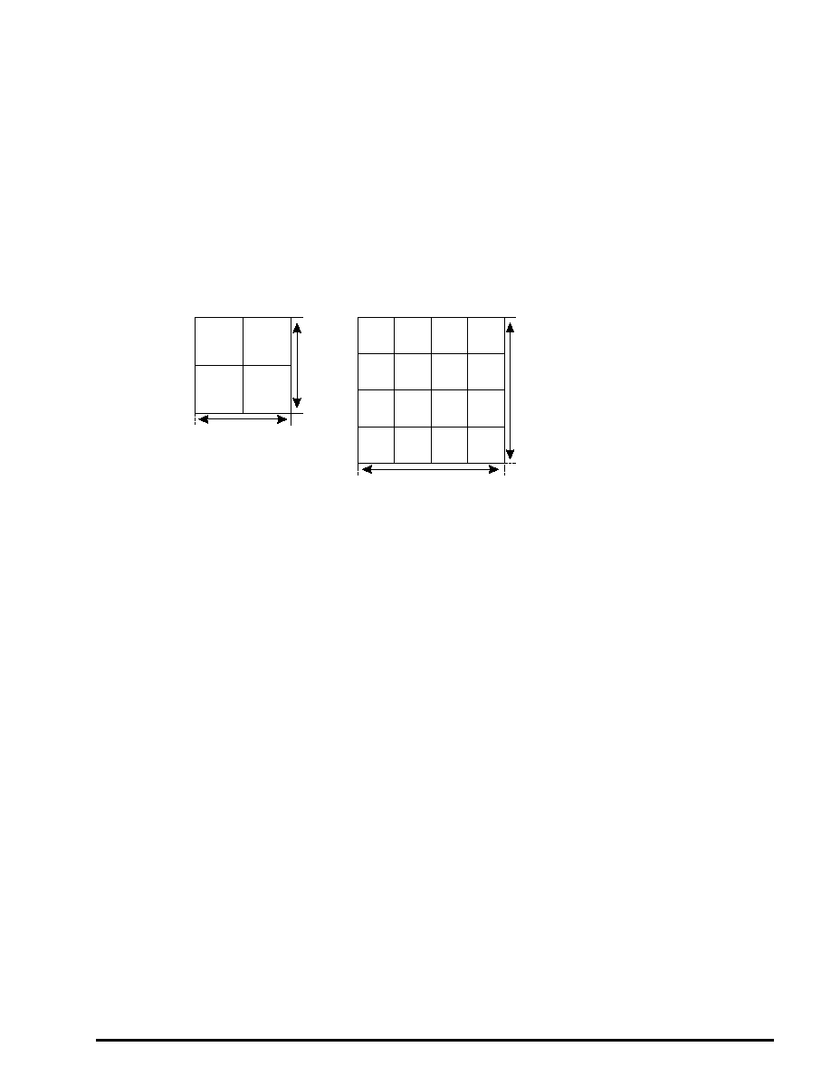
Programmer's Tutorial / Scrolls
8-21
Maps
Maps are the largest scroll unit actually used for scroll drawing in the SGL. For normal scroll
screens, a map consists of 2
×
2 planes (vertical
×
horizontal); for rotating scroll screens, a map
consists of 4
×
4 pages (vertical
×
horizontal).
The planes that make up a map can be freely determined by specifying the starting address of each
plane (actually the starting address where the pattern name data table that makes up the plane is
stored); in other words, it is not necessary for the planes to be stored consecutively in VRAM.
Therefore, it is possible to specify the same plane for all of the planes that make up the map.
In the scroll shift, enlargement/reduction and rotation operations described later, the shift and
transformations are all performed in map units.
Fig 8-14 Map Image
Plane A
Plane A
Plane I
Plane E
Plane M
Plane C
Plane K
Plane G
Plane O
Plane B
Plane J
Plane F
Plane N
Plane D
Plane L
Plane H
Plane P
Plane C
Plane B
Plane D
2 planes
4 planes
4 planes
2 planes
·
The map register specification
is made by specifying the starting
address for the pattern name
table for each plane.
a) Normal scrolls
b) Rotating scrolls
The map size is determined by the scroll screen type:
Normal scroll screens:
2
×
2 (horizontal
×
vertical) planes for a total of 4 planes
Rotating scroll screens: 4
×
4 (horizontal
×
vertical) planes for a total of 16 planes
In the SGL, the library functions "slMapNbg0 to 3" and sl1MapRA,RB" are used to register
each of the planes that make up a map.
[void slMapNbg0 to 3 (void *map_a, void *map_b, void *map_c, void *map_d);]
This function registers the plane data for each of the normal scroll screen maps.
For the parameters, substitute the starting addresses for each of the four planes to be regis-
tered. The target scroll screens are those whose normal scroll screen name corresponds with
the end of the function name.
[void sl1MapRA (void *map_a);]
[void sl1MapRB (void *map_a);]
These functions register the plane data for the rotating scroll screen map.
For each parameter, substitute the starting address of the plane to be registered. The function
registers 16 planes of data for the map, starting from the specified address.
In addition, the function "sl1MapRA" is used for map registration when rotation parameter
A was used, and "sl1MapRB" is used for map registration when rotation parameter B was
used.
Rotation parameters
For details on the rotation parameters, refer to the section on rotation parameters.
|

8-22
Programmer's Tutorial / Scrolls
Reduction setting
Of the five types of scroll screens in the Sega Saturn system, it is possible to enlarge or reduce
three of the screens: the rotating scroll screen "RGB0" and the normal scroll screens "NBG0" and
"NBG1". Of the three screens that permit enlargement or reduction, the rotating scroll screen
RBG0 permits enlargement or reduction at any ratio, while the normal scroll screens "NBG0" and
"NBG1" only permit reduction or enlargement by a factor ranging from 1/4 to 256.
In addition, in the case of normal scroll screens, there are three enlargement/reduction modes,
depending on the setting of the permitted range of reduction. This mode setting is called the
reduction setting, and this setting must be made when using the normal scroll screens "NBG0"
and "NBG1".
Table 8-13 Scroll Screen Enlargement/Reduction Ranges
Scroll type
Name
Enlargement/reduction
Enlargement/reduction
Normal scroll screen
NBG0
q
1/4 to 256x
NBG1
q
1/4 to 256x
NBG2
×
NBG3
×
Rotating scroll screen
RBG0
q
Any ratio
Note: For NBG0 and NBG1, the permitted range of reduction varies according to the reduction setting.
In the SGL, use the library function "slZoomModeNbg0,1" to make the reduction setting for the
corresponding normal scroll screen.
[void slZoomModeNbg0, 1 (Uint16 zoom_mode);]
This function determines the reduction setting for the normal scroll screens, either NBG0 or
NBG1, for which enlargement or reduction are possible.
The target scroll screen is the normal scroll screen with the same name as the end of the
function name.
For the parameters, substitute the value from the following chart corresponding to the reduc-
tion setting mode.
Table 8-14 slZoomModeNbg0,1 Substitution Values (zoom_mode)
Reduction setting
1x
1/2x
1/4x
Substitution value
ZOOM_1
ZOOM_HALF
ZOOM_QUARTER
Note: The values in the above table are defined by "sl_def.h".
Rotating scroll screen enlargement/reduction
Because the rotating scroll screen always permits enlargement or reduction at any
ratio, the reduction setting is not necessary.
Restriction on the number of scroll screens due to the reduction setting
The reduction setting for the normal scroll screens NBG0 and NBG1 (when set to permit
reduction to a smaller value) places restrictions on the number of scroll screens that can
be displayed and on their functions. This is because the reduction setting changes the
number of VRAM accesses that are made. For details on access restrictions, refer to
"HARDWARE MANUAL vol. 2: VDP2 User's Manual," pp. 31 to 42.
|

Programmer's Tutorial / Scrolls
8-23
Function settings unique to the rotating scroll screen (1)
In addition to the scroll function settings described up to this point, there are several function
settings that are necessary in the case of the rotating scroll screen.
These function settings are required in order to use the unique functions of the rotating scroll.
Rotation parameter setting:
When using the rotating scroll screen, an area for storing and calling the data concerning the
rotation is required; collectively, this data is called the "rotation parameters."
Therefore, when using the rotating scroll screen, it is necessary as part of the scroll function
settings to store the rotation parameters in VRAM. (Rotation parameter size: 100H) Use the
library function "slRparaInitSet" to specify the rotation parameters.
[void slRparaInitSet (ROTSCROLL *Rpara_adr);]
This function stores the rotation parameters in the VRAM area and simultaneously sets the
default values.
For the parameter, substitute the starting address of the area where the rotation parameters
are to be stored.
Rotation parameter usage mode:
There are two types of rotation parameters: A and B. These two types of rotation parameters
are stored together in an area that is allocated by using the function "slRparaInitSet". Because
there are two types of rotation parameters, two sets of status data are simultaneously retained for
rotating scrolls, one of which can be selected to draw the scroll on the monitor.
The user can select one of the following four rotation parameter usage modes in order to deter-
mine how the rotation parameters are to be used.
Mode 0: Use rotation parameters A
Mode 1: Use rotation parameters B
Mode 2: Switch the image according to the coefficient data read from the coefficient table in
rotation parameters A
Mode 3: Switch according to the rotation parameter window
[void slRparaMode (Uint16 mode);]
This function switches the rotation parameter usage mode.
For the parameter, substitute the flag in the following table that indicates the desired rotation
parameter usage mode.
Table 8-15 slRparaMode Parameter Substitution Values
Mode 0
Mode 1
Mode 2
Mode 3
Substitution value
RA
RB
K_CHANGE
W_CHANGE
Note: The actual values are defined in "sgl_def.h".
|

8-24
Programmer's Tutorial / Scrolls
Current Rotation Parameter Switching
Of the functions used for rotating scrolls, those functions whose names end in "R" set their
functions for the current rotation parameters; by using the function "slCurRpara" to switch the
current rotation parameters, it is possible to make separate function settings for rotation param-
eters A and B.
If a function name ends in "RA" or "RB", then that function makes a setting only for the rota-
tion parameters indicated by the end of the function name.
[void slCurRpara (Uint16 flag);]
Switches the current rotation parameters.
For the parameter, substitute the flag shown in the table below indicating the rotation param-
eters to be switched to.
Table 8-16 slCurRpara Substitution Values
Rotation parameters A
Rotation parameters B
Substitution value
RA
RB
Note: The actual values are defined in "sgl_def.h".
Note:
For details on the rotation parameters, refer to the "HARDWARE MANUAL vol. 2"
(VDP2 User's Manual: p. 151).
|

Programmer's Tutorial / Scrolls
8-25
Function settings unique to the rotating scroll screen (1)
Screen overflow processing mode selection:
This function selects the processing to be performed when the drawing of the rotating scroll
screen goes beyond the display area. This is called screen overflow processing. There are four
screen overflow processing modes:
Mode 0: The image set for the display area is repeated outside of the area.
Mode 1: The character pattern specified in the screen overflow PN register is repeated outside
of the display area.
Mode 2: The entire area outside of the display area is clear.
Mode 3: Clipping (0 _ X _ 512, 0 _ Y _ 512) is forcibly performed on the area, and the area
outside of the area is entirely clear.
Use the library function "slOverRA,RB" to select the screen overflow processing.
[void slOverRA (Uint16 over_mode);]
[void slOverRB (Uint16 over_mode);]
These functions select the screen overflow processing when the rotating scroll screen ex-
ceeds the display area.
For the parameter, substitute the value from the following table that corresponds to the
desired screen overflow processing mode.
The function "slOverRA" sets the overflow processing when rotation parameters A are used,
and the function "slOverRB" sets the overflow processing when rotation parameters B are
used.
Table 8-17 Screen Overflow Processing Parameter Substitution Values (over_mode)
Overflow processing mode
Mode 0
Mode 1
Mode 2
Mode 3
Parameter substitution value
0
1
2
3
|

8-26
Programmer's Tutorial / Scrolls
Scroll setting flow chart
The following flow chart summarizes the scroll setting procedure, including the setting of the
character patterns, the page -> plane -> map settings, the reduction setting, and scroll registra-
tion.
Flow Chart 8-1 Flow of Scroll Function Settings
START
Specify rotation
parameters (only when
using RBG0)
Select color
RAM mode
Set up pages
Set up maps
Specify character
pattern address
Register planes
in maps
Specify color
palette address
Specify data type for
pattern name data
Select reduction
setting
Select screen
overflow processing
Set up planes
Set rotation parameter
usage mode
Specify plane size
Scroll function
settings complete
Select scroll
function
Specify number
of colors
Set up character
patterns
Determine character
pattern size
Is the
target screen an NBG
screen?
No: RBG0
Yes: NBG0 - 3
|

Programmer's Tutorial / Scrolls
8-27
Scroll Drawing
This section explains the procedure from the point when the scroll function settings and scroll
registration have been completed up to the point where the scroll screen is actually drawn. The
explanation will describe the library functions in the sequence in which they are used.
Background screen setup
Background screen setup:
Select the color for the background screen.
The background screen is the single-color screen that is displayed in the background anywhere
on the monitor where nothing is displayed.
Use the library function "slBack1ColSet" to set the background screen.
[void slBack1ColSet (void *back_col_adr, Uint16 RGB_col);]
This function sets the background color for the single-color background screen.
For the parameters, set the starting address in VRAM where the background screen color
data is stored and a 1-word RGB value (#define value) that shows the background screen
color.
The #define value used for RGB color specification is defined in the header file "sl_def.h" as
"RGB_Flag".
Fig 8-15 RGB Color Mode Sample (RGB_Flag)
#define
#define
#define
#define
#define
#define
CD_Black
CD_DarkRed
CD_DarkGreen
|
|
|
CD_Purple
CD_Magenta
CD_White
(0<<10) | (0<<5) | (0) | RGB_Flag
(0<<10) | (0<<5) | (8) | RGB_Flag
(0<<10) | (8<<5) | (0) | RGB_Flag
(31<<10) | (0<<5) | (31) | RGB_Flag
(31<<10) | (31<<5) | (0) | RGB_Flag
(31<<10) | (31<<5) | (31) | RGB_Flag
·
·
RGB mode color sample
Note: The above values are defined in "sl_def.h".
|

8-28
Programmer's Tutorial / Scrolls
Display position setting
Normal scroll screen:
This function determines the display position of the normal scroll screen for which the function
has been set. Use the library function "slScrPosNbg0 to 3" to determine the normal scroll
screen display position.
[void slScrPosNbg0 to 3 (FIXED posx, FIXED posy);]
This function sets the normal scroll screen display coordinates.
For the parameters, substitute the values for the XY coordinates (in the scroll coordinate
system) that determine where the monitor will be positioned on the scroll map.
The normal scroll screen placement reference point is the upper left corner of the monitor.
Rotating scroll screen:
These functions determine the coordinates for the placement of the rotating scroll screen for
which the function has been set, as well as the coordinates for the center of rotation.
The function "slLookR" determines the display position of the rotating scroll screen, and the
function "slDispCenterR" determines the coordinates for the center of rotation.
[void slLookR (FIXED posx, FIXED posy);]
This function sets the rotating scroll screen placement coordinates and stores the information
in the current rotation parameters. For the parameters, specify the scroll XY coordinates that
will be the origin for the upper left corner of the scroll map. The display position of rotating
scrolls is determined by the placement coordinates and by the coordinates for the center of
rotation.
[void slDispCenterR (FIXED posx, FIXED posy);]
This function sets coordinates for the center of rotation (vanishing point) of the rotating
scroll screen and stores the information in the current rotation parameters. For the para-
meters, specify the screen XY coordinates where the rotating scroll screen is to be placed.
The display position of rotating scrolls is determined by the placement coordinates and by
the coordinates for the center of rotation.
Fig 8-16 Relationship between the Display Position and the Center of Rotation
Note:The positive direction on the
Z axis in the scroll screen is
towards the front of the screen.
Placement coordinate
Rotating scroll map
Coordinates
for center of
rotation
Monitor
Placement
Monitor
Rotating scroll map
Rotation
Monitor
Z axis rotation
Rotating scroll map
In addition, the functions "slLookR" and "slDispCenterR" can be used to make settings for the
rotation parameters A and B, respectively; use the function "slCurRpara" to switch between the
rotation parameters to be set (the rotation parameters currently being used). Of the functions
used for the rotating scrolls, all with a function name that ends with an "R" can be used to set
their corresponding functions independently for rotation parameters A and B.
|

Programmer's Tutorial / Scrolls
8-29
Scroll registration
Once all scroll data has been stored and all scroll function settings have been completed, it is
necessary to register the scroll by using the SGL library function "slScrAutoDisp". Scroll
registration is the process of setting up the cycle pattern and drawing settings for scroll screens
for which the function settings have been completed.
In addition, the scroll registration process may fail in some cases, depending on the scroll
function settings to be registered, the number of scroll screens, and the VRAM bank in which
the scroll data is stored. This is due to the various restrictions placed on scrolls, including
restrictions on scrolls due to the number of colors used in normal scroll screens as described
earlier. (These restrictions are discussed in the section that follows.)
[Uint16 slScrAutoDisp (Uint32 disp_bit);]
This function registers scroll screens for which functions have been set.
For the parameter, substitute the value from the following chart that corresponds to the scroll
screen to be registered.
The function returns a value of "0" if scroll registration is completed successfully, and of "-
1" if scroll registration fails.
Table 8-18 Scroll Registration Parameter Substitution Values (disp_bit)
Scroll screen to be registered
NBG0
NBG1
NBG2
NBG3
RBG0
Substitution value
NBG0ON
NBG1ON
NBG2ON
NBG3ON
RBG0ON
Note: The values in the above table are defined in "sl_def.h".
When registering more than one scroll screen, it is convenient to link the #define values corre-
sponding to each scroll screen by using the "or" ("|") operator when substituting for the param-
eter in the library function "slScrAutoDisp". (An example is shown in the diagram below.)
Fig 8-17 Multiple Scroll Screen Registration
Uint16 slScrAutoDisp(NBG0ON|NBG1ON|RBG0ON);
·
·
Multiple scroll screen registration
Note: The parameter substitution values are defined in "sl_def.h".
"or" operator
"or" operator
NBG0 registration
NBG0 registration
NBG1 registration
|

8-30
Programmer's Tutorial / Scrolls
Notes on scroll registration
When using the SGL library function "slScrAutoDisp" to perform scroll registration, in certain
cases the function may return a value of "-1". This return value indicates that the function
"slScrAutoDisp" failed at scroll registration.
There are four basic causes for scroll registration to fail:
Causes of scroll registration failure
1) Scroll restrictions due to the number of colors used in normal scroll screens
An attempt was made to register scroll screens which cannot be used due to the setting for
the number of colors used in NBG0 and NBG1.
2) Bank occupied by rotating scroll data
Rotating scroll screen data and normal scroll screen data were both stored in the same
VRAM bank.
3) Pattern name data storage bank limitations
Pattern name data is stored in both VRAM banks with names that end with the same number.
4) Deviation from allowable scroll functions
The scroll screen to be registered exceeded the number of scroll functions and screens that
can be selected at one time.
Measures to resolve each of these problems are described below.
Remedres for scroll registration faiture
Remedy for cause number 1:
Either decrease the number of colors set for NBG0 or NBG1, or else do not try to register
NBG2 or NBG3.
Remedy for cause number 2:
Store the scroll data for the rotating scroll screen and the normal scroll screen in separate
VRAM banks.
Remedy for cause number 3:
Observe the restrictions on storing pattern name data in VRAM banks.
Remedy for cause number 4:
Try reducing the number of scroll screens being registered, reducing the number of colors in the
character patterns in the function settings, increasing the reduction setting value, and reducing
the amount of scroll screen data in each VRAM bank.
VRAM access restrictions
The causes underlying number 4 above are ultimately caused by restrictions on ac-
cesses to VRAM banks. Explaining and comprehending the VRAM access restrictions
is very difficult. Therefore, we are limiting ourselves here to simply suggesting a
limitation of the number of scroll functions and screens as a means of solving this
problem.
(For details on VRAM access, refer to the " HARDWARE MANUAL vol. 2: VDP2
User's Manual.")
|
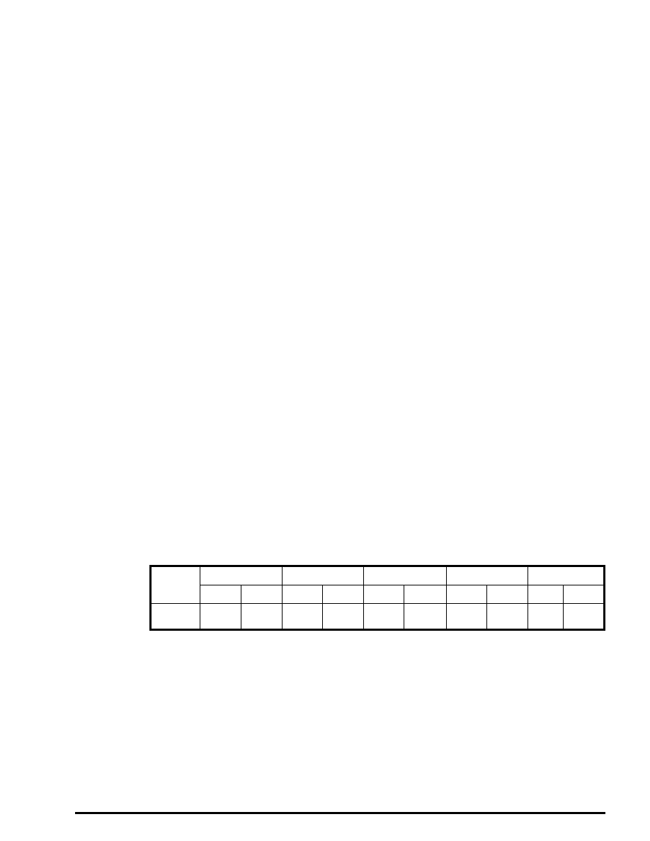
Programmer's Tutorial / Scrolls
8-31
Drawing start
Drawing declaration:
In the SGL, scroll screen drawing processing on the monitor screen begins for the first time
when the library function "slTVOn" is executed.
Subsequently, the scroll screens are drawn continuously on the screen in synchronization with
the scan lines according to the stored scroll information (position, scale, rotation angle, graphics
data, etc.).
In addition, there is also a complementary function to "slTVOn", called "slTVOff". This
function is used to halt scroll drawing processing.
[void slTVOn (void);]
This function starts drawing processing for scroll screens that have been set up for drawing.
[void slTVOff (void);]
This function halts drawing processing for scroll screens that have been set up for drawing.
Draw setup:
This setting determines whether or not a scroll screen for which the functions have been set is
actually drawn on the monitor or not. Scrolls which have been registered as scrolls by using the
function "slScrAutoDisp" have the draw setting set to "on" when they are registered, so draw-
ing of those scrolls is executed right away; however, it is possible to turn the draw setting off so
that the scrolls are not drawn. In addition, scrolls for which the draw setting has been turned off
can have the setting turned back on so that those scrolls are drawn again.
Operations involving scroll screens for which the draw setting has been turned off are not
executed.
[void slScrDisp (Uint32 mode);]
This function sets the draw setting for scroll screens for which the function settings have
been completed.
For the parameter, substitute the value from the table below corresponding to the draw
setting for each scroll screen.
Table 8-19 "slScrDisp" Parameter Substitution Value List (mode)
NBG0
NBG1
NBG2
NBG3
RBG0
ON
OFF
ON
OFF
ON
OFF
ON
OFF
ON
OFF
Substitution
NBG0ON
NBG0OFF NBG1ON
NBG1OFF
NBG2ON NBG2OFF
NBG3ON
NBG3OFF RBG0ON RBG0OFF
value
Note: The values in the above table are defined in "sl_def.h".
ON: Draw the scroll screen
OFF: Do not draw the scroll screen
Screen synchronization (scroll overwriting)
This function overwrites the scroll drawing data according to the state of the scan lines.
[void slSynch (void);]
This function overwrites the drawing data while the monitor is not overwriting the screen.
|

8-32
Programmer's Tutorial / Scrolls
Flow of operations up to scroll drawing
The following flow chart shows the flow of operations from the initialization of scroll data up to
the actual drawing of the scroll data, and serves as a summary of what has been explained up to
this point, from scroll function setup to scroll drawing.
Flow Chart 8-2 Flow of Operations up to Scroll Drawing
START
Initialize system
"slInitSystem"
Specify rotation parameters
(when using RGB0 only)
"slRparaInitSet"
Set screen overflow
processing
"slOverRA, RB"
Set background
screen
"slBack1ColSet"
Set screen overflow
processing
"slOverRA, RB"
Set scroll display
position
"slDispCenterR"
Store character pattern
data in VRAM
"Cel2VRAM"
Register scroll
"slScrAutoDisp"
Reduction setting
"slZoomModeNbg0, 1"
Set scroll display
position
"slScrPosNbg0 to 3"
Set rotation parameter
usage mode
"slParaMode"
Set rotation parameter
usage mode
"slParaMode"
Set rotation center
coordinates "slLookR"
Store pattern name
data in VRAM
"Map2VRAM"
Start drawing
"slTVOn"
Set up drawing
"slScrDisp"
Synchronize
screen "slSynch"
Store color data
in color RAM
"Pal2CRAM"
Set color RAM
mode "slColRam"
Set character patterns
"slCharNbg0 to 3,
slCharRbg0"
Set up pages
"slPageNbg0 to 3,
slPageRbg0"
Set up planes
"slPlaneNbg0 to 3,
slPlaneRA, RB"
Set up maps
"slMapNbg0 to 3,
slMapRA, RB"
Yes: NBG0
Yes: RBG0
Yes: RBG0
No: RBG0 - 3
No: NBG0 - 3
No: NBG0 - 3
Is scroll
screen RBG0?
Is scroll
screen RBG0?
Is scroll
screen RBG0?
Accessing VRAM and color RAM
If VRAM or color RAM is accessed during the monitor's display period, noise is gener-
ated on the monitor.
Therefore, accesses to these two RAM areas should either be made during a non-
display interval (during blanking) by using the function "slSynch", be made after
interrupting drawing processing by using the function "slTVOff", or else be made by
turning off the drawing setting with the function "slScrDisp" and then accessing the
VRAM bank not being accessed.
|

Programmer's Tutorial / Scrolls
8-33
Normal Scroll Screens
The normal scroll screens NBG0 to 3 permit vertical and horizontal movement of the scroll and
also expansion/reduction of the scroll (NBG0 and NBG1 only). These two functions are ex-
plained below via a sample program.
Normal scroll screen movement
The normal scroll screens NBG0 to NBG3 can be moved horizontally and vertically by chang-
ing the scroll display position.
This concept is illustrated below.
Fig 8-18 Scroll Display Position Concept
·
·
·
·
The scroll display position is processed
through the scroll screen coordinate system.
This coordinate system designates the
upper-left corner of each scroll or map as the
origin.
The scroll display position is specified by
indicating where in the coordinate system the
monitor should be positioned. (The representative
point is the upper-left corner of the monitor.)
As a result, if the scroll display position
coordinates are moved in the positive direction
along the X axis (to the right), the monitor
moves to the right on the scroll map, giving
the appearance that the scroll is moving to the left.
Normal scroll map
Move position
to right
Monitor
Monitor
b) Move to right
a) Initial state
The library function "slScrPosNbg0 to 3" is used to move the scroll display
position. "slScrPosNbg0 to 3" is also used to set the initial position of the scroll.
[void slScrPosNbg0 to 3 (FIXED posx, FIXED posy);]
This function sets the display start position for the normal scroll screens NBG0 to NBG3.
The scroll display position is determined by where the monitor is placed on the scroll map.
The upper left corner of the monitor is used as the representative point, and so only one point
is specified on the scroll map as a parameter.
For the parameter, specify the XY coordinates on the scroll coordinate system.
In addition, as the scroll display position moves up and down and left and right, if it goes
outside of the display area, the scroll wraps around from the other side.
Fig 8-19 Scroll Wraparound Processing
c) The excess portion is
drawn at the right edge
Monitor
Monitor
Monitor
Display area
Display area
Display area
a) Initial state
b) Display area has gone
beyond left edge
|

8-34
Programmer's Tutorial / Scrolls
The two sample programs that follow each use SGL library functions to move a scroll horizon-
tally and to move a scroll horizontally and vertically.
List 8-2 sample_8_8_1: Horizontal Scroll Movement
/*-----------------------------------------------------*/
/*
Graphic Scroll [X axis]
*
/*-----------------------------------------------------*/
#include
"sgl.h"
#include
"ss_scrol.h"
#define
NBG1_CEL_ADR
(VDP2_VRAM_B1+0x02000)
#define
NBG1_MAP_ADR
(VDP2_VRAM_B1+0x12000)
#define
NBG1_COL_ADR
(VDP2_COLRAM+0x00200)
#define
BACK_COL_ADR
(VDP2_VRAM_A1+0x1fffe)
void main()
{
FIXEDyama_posx=SIPOSX,yama_posy=SIPOSY;
slInitSystem(TV_320x224,NULL,1);
slTVOff();
slPrint("Sample program 8.8.1",slLocate(9,2));
slColRam(CRM16_1024);
slBack1ColSet(BACK_COL_ADR,0);
slCharNbg1(COL_TYPE-256,CHAR_SIZE_1x1);
slPageNbg1(NBG1_CEL_ADR,0,PNB_1WORD|CN_12BIT);
slPlaneNbg1(PL_SIZE_1x1);
slMapNbg1(NBG1_MAP_ADR,NBG1_MAP_ADR,NBG1_MAP_ADR,NBG1_MAP_ADR);
Cel2VRAM(yama_cel,NBG1_CEL_ADR,31808);
Map2VRAM(yama_map,NBG1_MAP_ADR,32,16,1,256);
Pal2CRAM(yama_pal,NBG1_COL_ADR,256);
slScrPosNbg1(yama_posx,yama_posy);
slScrAutoDisp(NBG1ON);
slTVOn;
while(-1){
slScrPosNbg1(yama_posx,yama_posy);
yama_posx+=POSX_UP;
slSynch();
}
}
/* screen mode setting */
/* drawing off */
/* color mode setting */
/* background screen setup */
/* scroll function setup */
/* scroll data storage */
/* initial display position setting */
/* scroll registration */
/* drawing start declaration */
/* scroll data overwrite */
/* screen synchronization */
/* include file containing various settings */
Note: The lightly shaded portion is defined in "sgl.h" and "sl_def.h".
Note: The darkly shaded portion is defined in "ss.scroll.h".
|

Programmer's Tutorial / Scrolls
8-35
Flow Chart 8-3 sample_8_8_1: Horizontal Scroll Movement
START
Initialize system
Set background
screen (single color)
Stop drawing
Set color mode
Set character
patterns
Store map
information in VRAM
Store cell
information in VRAM
Set up pages
Start drawing
Register scroll
Overwrite display position
change parameter
Reset scroll screen
display position
Synchronize
with screen
Store palette
information in color RAM
Set up planes
Set up maps
Set initial position
of scroll screen
|

8-36
Programmer's Tutorial / Scrolls
List 8-3 sample_8_8_2: Horizontal and Vertical Scroll MovementL
/*-----------------------------------------------------*/
/*
Graphic Scroll [X & Y axis]
*
/*-----------------------------------------------------*/
#include
"sgl.h"
#include
"ss_scrol.h"
#define
NBG1_CEL_ADR
(VDP2_VRAM_B1+0x02000)
#define
NBG1_MAP_ADR
(VDP2_VRAM_B1+0x12000)
#define
NBG1_COL_ADR
(VDP2_COLRAM+0x00200)
#define
BACK_COL_ADR
(VDP2_VRAM_A1+0x1fffe)
void main()
{
FIXED yama_posx=SIPOSX,yama_posy=SIPOSY;
Uint16scroll_flg=YOKO;
slInitSystem(TV_320x224,NULL,1);
TVOff();
slPrint("Sample program 8.8.2",slLocate(9,2));
slColRam(CRM16_1024);
slBack1ColSet(BACK_COL_ADR,0);
slCharNbg1(COL_TYPE_256,CHAR_SIZE_1x1);
slPageNbg1(NBG1_CEL_ADR,0,PNB_1WORD|CN_12BIT);
slPlaneNbg1(PL_SIZE_1x1);
slMapNbg1(NBG1_MAP_ADR,NBG1_MAP_ADR,NBG1_MAP_ADR,NBG1_MAP_ADR);
Cel2VRAM(yama_cel,NBG1_CEL_ADR,31808);
Map2VRAM(yama_map,NBG1_MAP_ADR,32,16,1,256);
Pal2CRAM(yama_pal,NBG1_COL_ADR,256);
slScrPosNbg1(yama_posx,yama_posy);
slScrAutoDisp(NBG0ON|NBG1ON);
slTVOn();
while(-1){
if(scroll_flg==YOKO){
if(yama_posx>=(SX*2+SIPOSX)){
scroll_flg=TATE;
yama_posx+SIPOSX;
}elseyama_posx+=POSX_UP;
}elseif(scroll_flg==TATE){
if(yama_posy>-(SY*2+SIPOSY)){
scroll_flg=YOKO;
yama_posy=SIPOSY;
}elseyama_posy+=POSY_UP;
}
siScrPosNbg1(yama_posx,yama_posy);
slSynch();
}
}
/* include file containing various settings */
/* screen mode setting */
/* drawing off */
/* color mode setting */
/* background screen setup */
/* scroll function setup */
/* scroll data storage */
/* initial display position setting */
/* scroll registration */
/* drawing start declaration */
/* scroll data overwrite */
/* screen synchronization */
Note: The lightly shaded portion is defined in "sgl.h" and "sl_def.h".
Note: The darkly shaded portion is defined in "ss.scroll.h".
|

Programmer's Tutorial / Scrolls
8-37
Flow Chart 8-4 sample_8_8_2: Horizontal and Vertical Scroll Movement
START
Initialize system
Set background
screen (single color)
Stop drawing
Set color mode
Set character
patterns
Store map
information in VRAM
Store cell
information in VRAM
Set up pages
Set initial position
of scroll
Register scroll
Start drawing
Overwrite display position
change parameter
Change scroll
flag to vertical
Change scroll
flag to horizontal
Set position X to
initial value
Set position Y to
initial value
Reset scroll screen
display position
Update position X
Update position Y
Synchronize
with screen
Store palette
information in color RAM
Set up planes
Set up maps
Does
scroll flag =
horizontal?
Has the
screen scrolled two circuits
horizontally?
Has the
screen scrolled two circuits
vertically?
No
No
No
Yes
Yes
Yes
|

8-38
Programmer's Tutorial / Scrolls
Normal scroll screen enlargement/reduction
Among the normal scroll screens, NBG0 and NBG1 can be enlarged or reduced. (Maximum
range: 1/4x to 256x) The following diagrams illustrate the concept.
Fig 8-20 Scroll Enlargement and Reduction
c) Reduced
Scroll
Monitor
Enlarged
Reduced
a) Initial state
b) Enlarged
When using the normal scroll screens NBG0 or NBG1, the possible range of reduction differs
depending on the reduction setting in the scroll function settings.
Table 8-20 Enlargement/reduction range depending on the reduction setting
Reduction setting
1x
1/2x
1/4x
Enlargement/reduction range
1x to 256x
1/2x to 256x
1/4x to 256x
In the SGL, in order to enlarge or reduce normal scroll screen NBG0 or NBG1, use the library
function "slZoomNbg0" or "slZoomNbg1", whichever corresponds to the scroll screen in
question.
[void slZoomNbg0, 1 (FIXED scale_x, FIXED scale_y);]
This function enlarges or reduces the normal scroll screen NBG0 or NBG1. For the param-
eters, substitute the reciprocals of the vertical and horizontal scroll ratios. For example, to
enlarge by a factor of 2, substitute "1/2" for the parameter; to reduce by 1/2, substitute "2"
for the parameter. The lower limit for the reduction range changes, depending on the reduc-
tion setting. (Refer to the above table.)
Enlargement/reduction function parameters settings:
When substituting for the parameters in the scroll enlargement/reduction function, it is
necessary to use the reciprocal of the desired ratio. (Ex,: To enlarge by a factor of 2,
substitute "1/2".)
The reason is that the values in the parameters do not show the scale value as is. The
values substituted for the enlargement/reduction function parameters show, after
displaying one dot of the scroll, the amount to move before displaying the next dot.
If the movement amount is specified as "2.0", the scroll skips one dot after displaying
each dot, with the result that the scroll is drawn at half size.
If the movement amount is 1.0, the resulting image scale is 1.0, and if the movement
amount is 2.0, the resulting image scale is 1/2; if the movement amount is 1/2, the same
dot is displayed twice, with the result that the displayed image becomes twice as big.
|

Programmer's Tutorial / Scrolls
8-39
The following sample program (List 8-4) shows how to use the SGL library functions to actu-
ally enlarge and reduce a normal scroll screen.
List 8-4 sample_8_8_3: Scroll Enlargement/Reduction
/*-----------------------------------------------------*/
/*
Graphic Scroll & Expansion & Reduction
*
/*-----------------------------------------------------*/
#include
"sgl.h"
#include
"ss_scrol.h"
#define
NBG1_CEL_ADR
VDP2_VRAM_B0
#define
NBG1_MAP_ADR
(VDP2_VRAM_B0+0x10000)
#define
NBG1_COL_ADR
(VDP2_COLRAM+0x00200)
#define
BACK_COL_ADR
(VDP2_VRAM_A1+0x1fffe)
void main()
{
FIXED yama_posx=toFIXED(0.0),yama_posy=toFIXED(0.0);
FIXED yama_zoom=toFIXED(1.0)
FIXED up_down=toFIXED(-0.1);
slInitSystem(TV_320x224,NULL,1);
slTVOff();
slPrint("Sample program 8.8.3",slLocate(9,2));
slColRAMMode(CRM16_1024);
slBack1ColSet(BACK_COL_ADR,0);
slCharNbg1(COL_TYPE_256,CHAR_SIZE_1x1);
slPageNbg1(NBG1_CEL_ADR,0,PNB_1WORD|CN_10BIT);
slPlaneNbg1(PL_SIZE_1x1);
slMapNbg1(NBG1_MAP_ADR,NBG1_MAP_ADR,NBG1_MAP_ADR,NBG1_MAP_ADR);
Cel2VRAM(yama_cel,NBG1_CEL_ADR,31808);
Map2VRAM(yama_map,NBG1_MAP_ADR,32,16,1,0);
Pal2CRAM(yama_pal,NBG1_COL_ADR,256);
slZoomModeNbg1(ZOOM_HALF);
slScrPosNbg1(yama_posx,yama_posy);
slScrAutoDisp(NBG1ON);
slTVOn();
while(-1){
if(yama_posx>=SX){
if(yama_zoom>=toFIXED(1.5))
up_down=toFIXED(-0.1)
elseif(yama_zoom<=toFIXED(0.7))
up_down=toFIXED(0.1)
yama_zoom+=up_down;
yama_posx=toFIXED(0.0);
slZoomNbg1(yama_zoom,yama_zoom);
}
siScrPosNbg1(yama_posx,yama_posy);
yama_posx+=POSX_UP;
slSynch();
}
}
/* include file containing various settings */
/* screen mode setting */
/* drawing off */
/* color mode setting */
/* background screen setup */
/* scroll function setup */
/* scroll data storage */
/* reduction setting */
/* initial display position setting */
/* scroll registration */
/* drawing start declaration */
/* scroll data overwrite */
/* scroll enlargement/reduction */
/* screen synchronization */
Note: The lightly shaded portion is defined in "sgl.h" and "sl_def.h".
Note: The darkly shaded portion is defined in "ss.scroll.h".
|

8-40
Programmer's Tutorial / Scrolls
Flow Chart 8-5 sample_8_8_3: Scroll Enlargement/Reduction
START
Initialize system
Stop drawing
Set scroll screen
display position
Set character
patterns
Reset scroll screen
display position
Reduction setting
Set background
screen (single color)
Reduce/enlarge
scroll screen
Store map
information in VRAM
Set color mode
Register scroll
Set up pages
Overwrite display
position change flag
Start drawing
Set up planes
Set up maps
Change rotation
angle
Synchronize
with screen
Store cell
information in VRAM
Store palette
information in color RAM
Has the
screen scrolled one circuit
horizontally?
Yes
No
|

Programmer's Tutorial / Scrolls
8-41
Rotating Scroll Screen
The rotating scroll screen RGB0 permits scroll enlargement/reduction and rotation. In addition,
unlike normal scroll screens, the scroll can be moved both in the horizontal and the vertical
directions, respectively.
In this section, these three functions (rotating scroll movement, enlargement/reduction, and
rotation) are explained in conjunction with a sample program.
Rotating scroll shift
Rotating scroll shifting is also actually realized by changing the scroll display position.
By using the "slLookR" function, it is possible to create the illusion that the scroll is moving up
and down or right and left across the monitor.
Fig 8-21 Rotating Scroll Movement
·
·
The rotating scroll display
position is determined by
the placement coordinates
and by the rotation center
coordinates.
To shift the rotating scroll,
fixing the rotation center
coordinates in place and
moving the placement
coordinates as shown in the
diagram at left, are sufficient
to move the rotating scroll.
Monitor
Monitor
Rotating scroll map
Rotating scroll map
Rotation
Rotating scroll screen enlargement/reduction
In the SGL, the enlargement/reduction operation can also be performed on the rotating scroll
screen. Unlike enlargement/reduction of normal scroll screens, enlargement/reduction of
rotating scroll screens can always be done at any desired ratio.
In addition, in the case of a rotating scroll screen, the scroll rotation operation described later,
the enlargement/reduction operation, and the movement operation can all be used together.
In the SGL, use the library function "slZoomR" to enlarge/reduce rotating scroll screens.
[void slZoomR (FIXED scale_x, FIXED scale_y);]
This function enlarges/reduces the rotating scroll screen RGB0, and saves the current state in
the current rotation parameters. (The current parameters can be switched by using the
"slCurRpara" function.)
For the parameters, substitute the reciprocals of the horizontal and vertical scroll ratios. For
example, to enlarge by a factor of 2, substitute "1/2" for the parameter; to reduce by 1/2,
substitute "2" for the parameter. In the case of the rotating scroll, the enlargement/reduction
ratio can always be set to any desired value.
|

8-42
Programmer's Tutorial / Scrolls
Rotating scroll screen rotation
In the Sega Saturn system, the rotating scroll screen can be rotated around any desired axis at
any desired angle. (The diagrams below illustrate the concept.)
Fig 8-22 Scroll Rotation Concept
c) 3D rotation
(X-Y axis rotation)
Scroll
Monitor
Rotation center coordinates
a) Initial state
b) 2D rotation
(Z axis rotation)
2D rotation (Z axis rotation)
In the SGL, use the library function "slZrotR" to perform the 2D rotation operation (Z axis
rotation) on the rotating scroll screen.
The point that is the center of rotation (one point on the scroll map) is the point that was set by
the library function "slDispCenterR".
[void slZrotR (ANGLE z_angle);]
This function rotates the rotating scroll screen RBG0 around the Z axis.
For the parameter, specify the Z axis rotation angle for the current rotation parameters.
Specify the rotation angle not as the angle from the current position, but as the absolute
angle. (The current parameters can be switched by using the "slCurRpara" function.)
The point set by the library function "slDispCenterR" is used as the center of rotation.
Fig 8-23 Actual Operation of Scroll Rotation
·
The rotation of the rotating scroll is
achieved by rotating the monitor
versus the scroll map.
Monitor
Monitor
Monitor
Rotating scroll map
Rotating scroll map
Rotation
Display
Z axis rotation: -45
°
Z axis rotation:
-45
°
Note on Function Usage
The functions "slZrotR", "slZoomR", and "slLookR" used for the rotating scroll
transformation operations cannot be used at the same time with the same rotation
parameters as the function "slScrMatSet" which performs the same transformation
operations on the rotating scroll.
This is because while the former group of functions overwrites a specific area in the
rotation parameters, the latter function overwrites the entire rotation parameter area.
|

Programmer's Tutorial / Scrolls
8-43
The following sample program (List 8-5) shows how to use the SGL library functions to actu-
ally rotate the rotating scroll screen.
List 8-5 sample_8_9_1: Scroll 2D Rotation
/*-----------------------------------------------------*/
/*
Graphic Rotation
*
/*-----------------------------------------------------*/
#include
"sgl.h"
#include
"ss_scrol.h"
#define
RBG0_CEL_ADR
VDP2_VRAM_A0
#define
RBG0_MAP_ADR
VDP2_VRAM_B0
#define
RBG0_COL_ADR
(VDP2_COLRAM+0x00200)
#define
RBG0_PAR_ADR
(VDP2_VRAM_A1+0x1fe00)
#define
BACK_COL_ADR
(VDP2_VRAM_A1+0x1fffe)
void main()
{
ANGLEyama_angz=DEGtoANG(0.0);
FIXEDposx=toFIXED(128.0),posy=toFIXED(64.0);
slInitSystem(TV_320x224,NULL,1);
slTVOff();
slPrint("Sample program 8.9.1",slLocate(9,2));
slColRAMMode(CRM16_1024);
slBack1ColSet(BACK_COL_ADR,0);
slRparaInitSet(RBG0_PAR_ADR);
slCharRbg0(COL_TYPE_256,CHAR_SIZE_1x1);
slPageRbg0(RBG0_CEL_ADR,0,PNB_1WORD|CN_10BIT);
slPlaneRA(PL_SIZE_1x1);
sl1MapRA(RBG0_MAP_ADR);
slOverRA(2);
Cel2VRAM(yama_cel,RBG0_CEL_ADR,31808);
Map2VRAM(yama_map,RBG0_MAP_ADR,32,16,1,0);
Pal2CRAM(yama_pal,RBG0_COL_ADR,256);
slDispCenterR(toFIXED(160.0),toFIXED(112.0));
slLookR(toFIXED(128.0),toFIXED(64.0));
slScrAutoDisp(RBG0ON);
slTVOn();
while(-1){
slZrotR(yama_angz);
yama_angz+=DEGtoANG(1.0);
slSynch();
}
}
/* include file containing various settings */
/* screen mode setting */
/* drawing off */
/* color mode setting */
/* background screen setup */
/* rotation parameter setting */
/* scroll function setup */
/* use rotation parameters A */
/* screen overflow processing */
/* scroll data storage */
/* initial display position setting */
/* scroll registration */
/* drawing start declaration */
/* scroll Z axis rotation */
/* screen synchronization */
Note: The lightly shaded portion is defined in "sgl.h" and "sl_def.h".
Note: The darkly shaded portion is defined in "ss.scroll.h".
|

8-44
Programmer's Tutorial / Scrolls
Flow Chart 8-6 sample_8_9_1: Scroll 2D Rotation
START
Initialize system
Set background
screen (single color)
Stop drawing
Set color mode
Set character
patterns
Store map
information in VRAM
Store cell
information in VRAM
Set up pages
Start drawing
Set LOOK
coordinates
Register scroll
Set center coordinates for
rotating scroll screen
Rotate around
Z axis
Synchronize
screen
Change rotation
angle
Store palette
information in color RAM
Set up planes
Set up maps
Set screen overflow
processing
|

Programmer's Tutorial / Scrolls
8-45
3D rotation using the current matrix
In the SGL, it is necessary to follow the procedure described below when performing a 3D
rotation operation (rotation around all axes) on the rotating scroll screen.
1) Rotating scroll setup
Complete all of the settings required when using the rotating scroll, such as the rotation
parameter settings, screen overflow processing, and coefficient table setup.
2) Coordinate operations
3D rotation operations involving the rotating scroll should first be executed against the
current matrix.
The same function group is used, namely, "slRotX", "slTranslate", "slScale", etc. However,
the sequence of operations (rotation, shift, and enlargement/reduction) is the opposite of that
for normal coordinate transformation operations. (Refer to chapter 4, "Coordinate Transfor-
mations," for details on the transformation operation sequence.)
In addition, the scroll coordinate system is a left-hand system in which the positive and
negative directions on the Z axis are reversed. However, because the conceptual image
entails rotating and moving the monitor versus the scroll, the resulting effect is actually the
same.
If you wish to perform coordinate transformation operations with the same matrix operation
procedure as used with normal coordinate transformation operations, use the function
"slScrMatConv" before the matrix data transfer. The function "slScrMatConv" converts the
current matrix that was transformed through the normal coordinate transformation proce-
dure, into a coordinate transformation matrix for scrolls and then makes the resulting matrix
into the current matrix.
[void slScrMatConv (void);]
This matrix converts the current matrix into coordinate transformation data for scrolls and
then replaces the current matrix with the results. Naturally, if this function is used on the
current matrix after executing the scroll coordinate transformation operation, the current
matrix is replaced with a matrix that can be used for normal coordinate transformations.
|

8-46
Programmer's Tutorial / Scrolls
3) Transferring the operation results to the rotation parameters
Next, transfer the results of the coordinate operations executed on the current matrix to the
rotation parameters. The rotating scroll is then altered and drawn according to the rotating
parameter data that was transferred.
Use "slScrMatSet" to transfer the data.
[void slScrMatSet (void));]
This function transfers the current matrix data to the current rotation parameters. Use for
transferring the current matrix on which the coordinate transformation operation for the
rotating scroll has been performed.
Flow Chart 8-7 3D Rotation Operation Procedure Using the current Matrix
START
Set rotation parameters
"slRparaInitSet"
Set rotation parameter
usage mode "slRparaMode"
Make scroll
settings
Set screen overflow
processing
"slOverRA" "slOverRB"
Set rotation center
"slDispCenterR"
Start drawing
Make drawing settings
"slAutoDisp", etc.
Specify rotation
parameters "slCurRpara"
Place scroll
"slLookR"
Transfer operation
results to rotation
parameters "slScrMatSet"
Synchronization
"slSynch"
Execute coordinate
operations on current
matrix "slRotX", etc.
|

Programmer's Tutorial / Scrolls
8-47
Controlling the zoom ratio by using the coefficient table
When executing a 3D rotation operation on the rotating scroll, the scroll is scaled according to
its "depth" in the screen. Normally, this scaling ratio is calculated on the basis of the param-
eters used in 3D coordinate operations, such as perspective transformations and then the results
are used to reshape the scroll; it is possible, however, to set this reshaping ratio for the indi-
vidual lines or dots beforehand and then use these ratios when reshaping the scroll. These ratios
as a group are called the "coefficient table."
The following two functions are needed when using the coefficient table.
1) Coefficient table creation:
First, it is necessary to allocate an area in VRAM for the coefficient table. The coefficient
table must be created in VRAM. In addition, the coefficient table will occupy one bank in
VRAM. This is because the coefficient table references the VRAM area at the maximum
access rate (8 times) for one bank.
[void slMakeKtable (void *adr);]
This function creates the coefficient table to be used in the 3D rotation operations at the
specified address. For the parameter, substitute the starting address of the area where the
coefficient table is to be created. The coefficient table must always be allocated in VRAM.
2) Coefficient table usage mode setting
When using the area that was specified as the coefficient table, this function determines the
usage mode, which indicates how the coefficient table is to be used.
[void slKtableRA, RB (void *table_adr, Uint16 mode);]
This function specifies the address of the coefficient table to be used, and also determines
which of the contents of the coefficient table are to be used. For the parameters, substitute
the starting address of the coefficient table, and also values (which can be connected by
using the "or" operator "|") from the following figure indicating coefficient table usage
modes.
The function "slKtableRA" sets the coefficient table for rotation parameters A, and
"slKtableRB" sets the coefficient table for rotation parameters B.
Fig 8-24 slKtableRA, RB Parameter Substitution Values (mode)
Table usage:
Coefficient data size:
Coefficient mode:
Line color:
Reshaping unit:
Fixed coefficients:
[K_OFF | K_ON ]|
[K_2WORD | K_1WORD ]|
[K_MODE0 | K_MODE1 | K_MODE2 | K_MODE3 ]|
[K_LINECOL ]|
[K_DOT | K_LINE ]|
[K_FIX ]|
·
·
slKtableRA, RB substitution values
Note: If "fixed coefficients" is specified as a parameter, the coefficient table is
assumed to have been created beforehand, and the coefficient table is not
executed in real time.
Note:
For details on coefficient tables, refer to "HARDWARE MANUAL vol. 2: VDP2, p. 163."
|

8-48
Programmer's Tutorial / Scrolls
List 8-6 sample_8_9_2: 3D Rotation
#include
"sgl.h"
#include
"ss_scrol.h"
#define
RBG0RB_CEL_ADR
VDP2_VRAM_A0
#define
RBG0RB_MAP_ADR
VDP2_VRAM_B0
#define
RBG0RB_COL_ADR
(VDP2_COLRAM+0x00200)
#define
RBG0RA_CEL_ADR
(RBG0RB_CEL_ADR+0x06e80)
#define
RBG0RA_MAP_ADR
(RBG0RB_MAP_ADR+0x02000)
#define
RBG0RA_COL_ADR
(RBG0RB_COL_ADR+0x00200)
#define
RBG0_KTB_ADR
VDP2_VRAM_A1
#define
RBG0_PRA_ADR
(VDP2_VRAM_A1+0x1fe00)
#define
RBG0_PRB_ADR
(RBG0RB_PRA_ADR+0x00080)
#define
BACK_COL_ADR
(VDP2_VRAM_A1+0x1fffe)
void main()
{
FIXED
posy=toFIXED(0.0);
ANGLE
angz=DEGtoANG(0.0);
ANGLE
angz_up=DEGtoANG(0.0);
slInitSystem(TV_320x224,NULL,1);
slTVOff();
slPrint("Sample program 8.9.2",slLocate(9,2));
slColRam(CRM16_1024);
slRparaInitSet(RBG0_PRA_ADR);
slMakeKtable(RBG0_KTB_ADR);
slCharRbg0(COL_TYPE_256,CHAR_SIZE_1x1);
slPageRbg0(RBG0RB_CEL_ADR,0,PNB_1WORD|CN_12BIT);
slPlaneRA(PL_SIZE_1x1);
sl1MapRA(RBG0_MAP_ADR);
slOverRA(0);
slKtableRA(RBG0_KTB_ADR,K_FIX|K_DOT|K_2WORD|K_ON);
Cel2VRAM(tuti_cel,RBG0RA_CEL_ADR,65536):
Map2VRAM(tuti_map,RBG0RA_MAP_ADR,64,64,2,884);
Pal2CRAM(tuti_pal,RBG0RA_COL_ADR,160);
slPlaneRB(PL_SIZE_1X1);
slMapRB(RBG0RB_MAP_ADR);
slOverRB(0);
Cel2VRAM(sora_cel,RBG0RB_CEL_ADR,28288);
Map2VRAM(sora_map,RBG0RB_MAP_ADR,64,20,1,0);
Pal2VRAM(sora_pal,RBG0RB_COL_ADR,256);
slRparaMode(K_CHANGE);
slBack1ColSet(BACK_COL_ADR,0);
slScrAutoDisp(RBG0ON);
slTVOn();
while(1)
{
slCurRpara(RA);
slUnitMatrix(CURRENT);
slTranslate(toFIXED(0.0),toFIXED(0.0)+posy,toFIXED(100.0));
posy-=toFIXED(5.0);
slRotX(DEGtoANG(-90.0));
slRotZ(angz);
slScrMatSet();
slCurRpara(RB);
slUnitMatrix(CURRENT);
slTranslate(toFIXED(160.0),toFIXED(155.0),toFIXED(100.0);
slRotZ(angz);
slScrMatSet();
angz_up+=DEGtoANG(0.5);
angz=(slSin(angz_up)>>4):
slSynch();
}
}
/* include file containing various settings */
/* screen mode setting */
/* drawing off */
/* color mode setting */
/* rotation parameter setting */
/* coefficient table setup */
/* screen overflow processing (RA) */
/* scroll data storage (RA) */
/* screen overflow processing (RB) */
/* scroll data storage (RB) */
/* rotation parameter usage mode setting
/* background screen setup */
/* scroll registration */
/* drawing start declaration */
/* scroll 3D rotation */
/* use rotation parameters A */
/* scroll Z axis rotation */
/* use rotation parameters B */
/* screen synchronization */
Note: The lightly shaded portion is defined in "sgl.h" and "sl_def.h".
Note: The darkly shaded portion is defined in "ss.scroll.h".
|

Programmer's Tutorial / Scrolls
8-49
Flow Chart 8-8 sample_8_9_2: 3D Rotation
START
Initialize system
Set up planes
(RB)
Change current
rotation parameters
Change current
rotation parameters
Set up pages
Register scroll
Update Z axis
rotation angle
Transfer current matrix
to rotation parameters
Specify rotation parameter
table address
Store scroll data
(for parameter B)
Update position
Update position
Set screen overflow
processing (RA)
Stop drawing
Set up maps
(RB)
Change current
matrix to unit matrix
Change current
matrix to unit matrix
Set up planes
(RA)
Start drawing
Synchronize
screen
Create coefficient
table
Set rotation
parameter mode
Z axis rotation
X axis rotation
Set coefficient
table usage mode
Set color mode
Set screen overflow
processing (RB)
Set position
Set position
Set up maps
(RA)
Set character
patterns
Set background
screen
Transfer current matrix
to rotation parameters
Z axis rotation
Store scroll data
(for parameter A)
LOOP
|

8-50
Programmer's Tutorial / Scrolls
Special Scroll Functions
In the Sega Saturn system, several special scroll functions are provided in addition to the normal
scroll functions. Of these, the SGL supports the ASCII scroll function and the transparent color
bit control function.
ASCII scrolls
The ASCII scroll function uses data called "ASCII cells" as the character pattern data in place
of normal scroll character pattern data. ASCII cells are normal ASCII data (ABCDEFG...) that
has been converted into a data format (cell data) that can be used by scrolls. This concept is
illustrated below.
Fig 8-25 ASCII Scrolls
·
·
An ASCII scroll uses ASCII data
as the scroll data.
Half-sized alphanumerics can be
drawn continuously, and the
sequence is the same as the
sequence of the ASCII codes.
Monitor
In the SGL, the ASCII cells are stored in VRAM during system initialization. ASCII scrolls can
be used by using this data in normal scroll function settings.
When the system is initialized, an ASCII scroll consists of 128 cells and 256 colors, and is set to
use the normal scroll screen NBG0.
The ASCII scroll data is stored in the following RAM areas:
Character data:
2000H starting from address 0x25e76000
Map data:
1000H starting from address 0x25e60000
Palette data:
20H starting from address 0x25f00000
Note: If, for some reason, other scroll data is later written to the above areas, the
ASCII scroll data will be overwritten by the new data, with the result that the default
ASCII scroll data will no longer be available.
|

Programmer's Tutorial / Scrolls
8-51
The following sample program (List 8-7) draws an ASCII scroll on the TV screen.
List 8-7 sample_8_10_1: ASCII Scrolls
/*-----------------------------------------------------*/
/*
Ascii Scroll
*/
/*-----------------------------------------------------*/
#include
"sgl.h"
#include
"ss_scrol.h"
#define
NBG1_CEL_ADR
VDP2_VRAM_B1
#define
NBG1_MAP_ADR
(VDP2_VRAM_B1+0x18000)
#define
NBG1_COL_ADR
VDP2_COLRAM
#define
BACK_COL_ADR
(VDP2_VRAM_A1+0x1fffe)
void main()
{
FIXEDascii_posx=SIPOSX,ascii_posy=SIPOSY;
slInitSystem(TV_320x224,NULL,1);
slTVOff();
slPrint("Sample program 8.10.1",slLocate(9,2));
slColRAMMode(CRM16_1024);
slBack1ColSet(BACK_COL_ADR,0);
slCharNbg1(COL_TYPE_256,CHAR_SIZE_1x1);
slPageNbg1(NBG1_CEL_ADR,0,PNB_1WORD|CN_10BIT);
slPlaneNbg1(PL_SIZE_1x1);
slMapNbg1(NBG1_MAP_ADR,NBG1_MAP_ADR,NBG1_MAP_ADR,NBG1_MAP_ADR);
Map2VRAM(ascii_map,NBG1_MAP_ADR,32,4,0,0);
slScrAutoDisp(NBG0ON|NBP1ON);
slTVOn();
while(1){
slScrPosNbg1(ascii_posx,ascii_posy);
ascii_posx+=POSX_UP;
slSynch();
}
}
/* include file containing various settings */
/* screen mode setting */
/* drawing off */
/* color mode setting */
/* background screen setup */
/* scroll function setup */
/* scroll data storage */
/* scroll registration */
/* drawing start declaration */
/* scroll placement */
/* screen synchronization */
Note: The lightly shaded portion is defined in "sgl.h" and "sl_def.h".
Note: The darkly shaded portion is defined in "ss.scroll.h".
|

8-52
Programmer's Tutorial / Scrolls
Flow Chart 8-9 sample_8_10_1: ASCII Scrolls
START
Initialize system
Set background screen
(single color)
Stop drawing
Set color mode
Set character
patterns
Set up planes
Store map information
in VRAM
Set up pages
Set up maps
Reset scroll screen
display position
Overwrite display
position change flag
Register scroll
Start drawing
|

Programmer's Tutorial / Scrolls
8-53
Transparent color bits
In the Sega Saturn, when palette format is selected for the scroll color data, the first (No. 0)
color data in one palette can be specified as transparent color, regardless of the previously
registered color data.
The transparent color is a color specification that when dots are specified as having the transpar-
ent color, processing is performed to determine if the transparent specification is on, and if it is,
the display of graphics such as a scroll that are behind a scroll for which the transparent color
specification was made are given priority. This concept is illustrated in the diagrams below.
Fig 8-26 Conceptual Model of Transparency Setting
c-2) Image when transparent
processing is on
Composition and drawing
Normal color
Color for which transparent
processing would be executable
·
·
In c-1, because transparent processing
is not being executed, the 3D polygon in
the background is not drawn.
In c-2, because transparent processing
is being executed, the transparent color
portion (palette selection No. 0) becomes
transparent, and the 3D polygon in the
background is drawn.
a) 3D polygon screen (background)
b) Scroll screen (foreground)
c-1) Image when transparent
processing is off
In the SGL, use the library function "slScrTransparent" to use the transparent color function.
Subsequent to the use of the "slScrTransparent" function, scrolls are drawn according to the
specification.
[void slScrTransparent (Uint16 trns_flag);]
When the palette format is selected for the scroll color data, this function selects whether or
not to perform transparent processing on palette selection number 0 in the palette data.
For the parameter, substitute the value from the following chart corresponding to the scroll
screen for which transparent processing is to be executed. Transparent processing can be
specified for multiple scroll screens by stringing together multiple parameters with the "or"
("|") operator.
Table 8-21 "slScrTransparent" Parameter Substitution Values (trns_flag)
Scroll screen for which transparent processing is to be executed
NBG0
NBG1
NBG2
NBG3
RBG0
Substitution value
NBG0ON
NBG1ON
NBG2ON
NBG3ON
RBG0ON
Note: The values in the table above are defined in "sl_def.h", which is included with the system.
The following sample program (List 8-8) demonstrates transparent color processing with scrolls
using the SGL library function "slScrTransparent".
|

8-54
Programmer's Tutorial / Scrolls
List 8-8 sample_8_10_2: Transparent Code Control
/*-----------------------------------------------------*/
/*
Priority Control
*/
/*-----------------------------------------------------*/
#include
"sgl.h"
#include
"ss_scrol.h"
#define
NBG1_CEL_ADR
VDP2_VRAM_B0
#define
NBG1_MAP_ADR
(VDP2_VRAM_B0+0x10000)
#define
NBG1_COL_ADR
(VDP2_COLRAM+0x00200)
#define
NBG2_CEL_ADR
(VDP2_VRAM_B1+0x02000)
#define
NBG2_MAP_ADR
(VDP2_VRAM_B1+0x12000)
#define
NBG2_COL_ADR
(VDP2_ COLRAM+0x00400)
#define
BACK_COL_ADR
(VDP2_VRAM_A1+0x1fffe)
void main()
{
Uint16trns_flg=NBG1ON;
FIXED yama_posx=SIPOSX,yama_posy=SIPOSY;
FIXED am2_posx=SIPOSX,am2_posy=SIPOSY;
slInitSystem(TV_320x224,NULL,1);
slTVOff();
slPrint("Sample program 8.10.2",slLocate(9,2));
slColRam(CRM16_1024);
slBack1ColSet(BACK_COL_ADR,0);
slCharNbg1(COL_TYPE_256,CHAR_SIZE_1x1);
slPageNbg1(NBG1_CEL_ADR,0,PNB_1WORD|CN_10BIT);
slPlaneNbg1(PL_SIZE_1x1);
slMapNbg1(NBG1_MAP_ADR,NBG1_MAP_ADR,NBG1_MAP_ADR,NBG1_MAP_ADR);
Cel2VRAM(am2_cel,NBG1_CEL_ADR,16000);
Map2VRAM(am2_map,NBG1_MAP_ADR,32,32,1,0);
Pal2CRAM(am2_pal,NBG1_COL_ADR,256);
slCharNbg2(COL_TYPE_256,CHAR_SIZE_1x1);
slPageNbg2(NBG2_CEL_ADR,0,PNB_1WORD|CN_12BIT);
slPlaneNbg2(PL_SIZE_1x1);
slMapNbg2(NBG2_MAP_ADR,NBG2_MAP_ADR,NBG2_MAP_ADR,NBG2_MAP_ADR);
Cel2VRAM(yama_cel,NBG2_CEL_ADR,31808);
Map2VRAM(yama_map,NBG2_MAP_ADR,32,16,2,256);
Pal2CRAM(yama_pal,NBG2_COL_ADR,256);
slScrPosNbg2(yama_posx,yama_posy);
slScrPosNbg1(am2_posx,am2_posy);
slScrTransparent(trns_flg);
slScrAutoDisp(NBG1ON|NBG2ON);
slTVOn;
while(1){
if(yama_posx>=(SX+SIPOSX)){
if(trns_flg==NBG1ON)
trns_flg=NBG1OFF;
else
trns_flg=NBG1ON;
yama_posx+SIPOSX;
slScrTransparent(trns_flg);
}
slScrPosNbg2(yama_posx,yama_posy);
yama_posx+=POSX_UP;
slScrPosNbg1(am2_posx,am2_posy);
am2_posy+=POSY_UP;
slSynch();
}
}
/* include file containing various settings */
/* screen mode setting */
/* drawing off */
/* color mode setting */
/* background screen setup */
/* scroll function setup */
/* NBG1 */
/* scroll function setup */
/* NBG2 */
/* initial display position setting */
/* scroll registration */
/* drawing start declaration */
/* scroll data overwrite */
/* change transparent enable bit */
/* screen synchronization */
Note: The lightly shaded portion is defined in "sgl.h" and "sl_def.h".
Note: The darkly shaded portion is defined in "ss.scroll.h".
|

Programmer's Tutorial / Scrolls
8-55
Flow Chart 8-10 sample_8_10_2: Transparent Code Control
START
Initialize system
Set character
patterns (scroll 2)
Stop drawing
Set up pages
(scroll 2)
Set character
patterns (scroll 1)
Store cell
information in VRAM
Store map
information in VRAM
Reset scroll screen
1 display position
Set background
screen (single color)
Set up maps
(scroll 2)
Enable transparent
processing
Set color mode
Set up planes
(scroll 2)
Set up pages
(scroll 1)
Store cell
information in VRAM
Make initial setting of transparent
display enable function
Overwrite display
position change
parameter (screen 1)
Overwrite display
position change
parameter (screen 2)
Synchronize
screen
Set up planes
(scroll 1)
Store palette
information in color RAM
Store map
information in VRAM
Register scroll
Start drawing
Set up maps
(scroll 1)
Set initial positions
of scroll screens
Store palette information
in color RAM
Reset scroll screen
2 display position
Has scroll
completed one horizontal
circuit?
Yes
No
|

8-56
Programmer's Tutorial / Scrolls
Color calculations
In the SGL, it is possible to compare the priority of sprites and each scroll screen and perform
calculations on the color data for the top image and the second image in the specified propor-
tions and display the result on the screen.
Using this function, it is possible to have a scroll screen or sprite hidden behind another scroll to
gradually fade into view.
The following procedure is required in order to perform color calculation processing.
1) Color calculation processing settings
Use the function "slColorCalc" to make the various settings for color operation processing,
and use the function "slColorCalcOn" to determine the scroll screens that are to be affected
by color calculations.
[void slColorCalc (Uint16 flag);]
This function makes the various settings needed for color calculation processing.
For the parameters, substitute the values from the following table corresponding to the color
calculation processing controls to be used.
For details on the parameters, refer to Chapter 12, "Color Operations," in Hardware Manual
vol.2: VDP2."
Fig 8-27 slColorCalc Substitution Values (flag)
Calculation method:
Image for which calculation is specified:
Extended color calculations:
Registered screen:
[CC_RATE| CC_ADD ]|
[CC_TOP | CC_2ND ]|
[CC_EXT ]|
[NBG0|NBG1|NBG2|NBG3|RBG0|LNCLON|SPRON]|
·
·
ColorCalc Substitution Values
Note: The above values are defined in "sl_def.h" provided with the system.
There are basically two color calculation modes.
Proportional addition: Perform color calculation with specified calculation ratio between the
top image and the second image. (CC_RATE)
Direct addition:
Perform color calculation simply by adding the top image and the
second image together. (CC_ADD)
[void slColorCalcOn (Uint16 flag);]
This function determines the scroll screens that are affected by color calculation processing.
For the parameters, substitute the values form the table below corresponding to the scroll
screens for which color calculations are to be performed. Color calculation can be specified
for multiple scroll screens at the same time by stringing together multiple parameters with
the "or" ("|") operator.
Table 8-22 slColorCalcOn Parameter Substitution Values (flag)
Scroll screen for which color calculations are to be executed
NBG0
NBG1
NBG2
NBG3
RBG0
LNCL
SPRITE
Substitution value
NBG0ON
NGB1ON
NBG2ON
NBG3ON
RBG0ON
LNCLON
SPRON
Note: The values in the table above are defined in "sl_def.h".
|

Programmer's Tutorial / Scrolls
8-57
2) Setting the color calculation values
Once the color calculation settings and registration process have been completed for the
scroll screens, the actual color calculation processing can be executed (specified by propor-
tion) on the scroll screens by using the functions "slColRateNbg0 to 3", "slColRateRbg0",
"slColRateLNCL" and "slColRateBACK".
However, the proportion specification has no meaning in cases where the addition method is
adopted for the color calculations.
[void slColRateNbg0 to 3 (Uint16 rate);]
[void slColRateRbg0 (Uint16 rate);]
[void slColRateLNCL (Uint16 rate);]
[void slColRateBACK (Uint16 rate);]
These functions set the color calculation ratios for the scroll screens specified by the func-
tions. For the parameters, substitute the color calculation ratio (range: 0 to 31) to be used in
the color calculation. The function "slColRateNbg0 to 3" is used to set the color calculation
ratio for each normal scroll screen, the function "slColRateRbg0" is used to set the color
calculation ratio for the rotating scroll screen, the function "slColRateLNCL" is used to set
the color calculation ratio for line color screens, and the function "slColRateBACK" is used
to set the color calculation ratio for the background screen.
The flow of color calculation processing is summarized in the flow chart below.
Flow Chart 8-11 Flow of Color Calculation Processing
START
Set up scrolls
Set up color calculations
"slColorCalc"
Register color calculations
"slColorCalcOn"
Set color calculation ratio
"slColRateNbg0 to 3", etc.
Synchronize screen
"slSynch"
Specify color
calculation addition
Set up drawing
|

8-58
Programmer's Tutorial / Scrolls
Line color screen
The line color screen is a special scroll screen provided specifically to be forcibly inserted as a
second image behind the top image (the image actually displayed on the monitor) on the speci-
fied scroll screen.
The line color screen permits the setting of a color for either the entire screen or for each line of
the screen.
It is necessary to store the collection of color RAM address data for the colors used for each line
as a line color table in VRAM.
Note: For details on the line color screen, refer to "Line Screen," in the "HARDWARE
MANUAL vol. 2:VDP2."
The procedure described below must be followed in order to use the line color screen.
1) Line color screen setup
When using the line color screen, it is first necessary to specify the line color table in which
the line color data is to be stored.
Also, do not forget to store in color RAM the color data specified in the line color table.
[void slLineColTable (void *adr);]
This function specifies the line color table address.
For the parameter, specify the address in VRAM where the line color table is to be stored.
To use only a single color on the line color screen, use the function "slLine1ColSet".
[void slLine1ColSet (void *adr, Uint16 col);]
This function sets the line color screen to a single color.
For the parameters, substitute the starting address of the area where the line color table is to
be stored, and also the color number of the desired color.
2) Scroll screen registration
Next, register the scroll screens that will be affected by the line color screen.
Use the function "slLineColDisp" to register scroll screens.
[void slLine1ColDisp (Uint16 flag);]
This function determines the scroll screens that will be affected by the line color screen.
For the parameters, substitute the values from the following table that correspond with the
scroll screens to be registered.
Multiple scroll screens can be registered by stringing together multiple parameters with the
"or" ("|") operator.
Table 8-23 slLineColDisp Parameter Substitution Values (flag)
Scroll screen to be registered
NBG0
NBG1
NBG2
NBG3
RBG0
Substitution value
NBG0ON
NBG1ON
NBG2ON
NBG3ON
RBG0ON
Note: The above values are defined in "sl_def.h" provided with the system.
|

Programmer's Tutorial / Scrolls
8-59
3) Color calculations using the line color screen
Scroll screens which have been registered with the function "slLineColDisp" can be used in
color calculation processing with the line color screen when used in conjunction with the
color calculation processing settings described earlier. For details on color calculation
processing, refer to the previous item, "Color calculations."
Flow Chart 8-12 Flow of Line Color Screen Processing
START
Set up scrolls
Specify line color table
"slLineColTable"
Specify single color
for line color screen
"slLine1ColSet"
Color calculation
processing
"slColRateLNCL"
Synchronize screen
"slSynch"
Register affected screens
"slLineColDisp"
|

8-60
Programmer's Tutorial / Scrolls
Color offset
In the SGL, it is possible to change the colors displayed on the screen by adding or subtracting
an offset value to the color RAM data (without changing the actual value) for sprites and each
scroll screen.
The procedure described below must be followed in order to use the color offset function.
1) Color offset setup
There are two color offsets: A and B.
To use the color offset function with a scroll screen, it is necessary to register the scroll
screen with one of the two color offsets.
To register scrolls, use the functions "slColOffsetOn" and "slColOffsetBUse".
[void slColOffsetOn (Uint16 flag);]
This function registers a scroll screen with the color offset function.
For the parameter, substitute a value from the table below corresponding to the scroll screen
to be registered.
[void slColOffsetBUse (Uint16 flag);]
This function registers scroll screens to be used with color offset B.
Scroll screens registered with just function "slColOffsetOn" use offset A. For the parameter,
substitute a value from the table below corresponding to the scroll screen to be registered.
Table 8-24 "slColOffsetOn", "slColOffsetBUse" Parameter Substitution Values (flag)
Scroll screen to be registered
NBG0
NBG2
NBG3
RBG0
BACK
SPRITE
Substitution value
NBG0ON
NBG2ON
NBG3ON
RBG0ON
BACKON
SPRON
Note: The above values are defined in "sl_def.h".
2) Setting the offset values
The scroll screens that have been registered are displayed with the effects of the color offset
in place.
Use the function "slColOffsetA, B" to set the color offset values.
[void slColOffsetA (Sint16 r, Sint16 g, Sint16 b);]
[void slColOffsetB (Sint16 r, Sint16 g, Sint16 b);]
These functions set the color offset values.
For the parameters, substitute the offset values (9 bits, signed) for red, green, and blue.
Use the function "slColOffsetA" to set the color offset values A, and the function "slColOffsetB"
to set the color offset values B.
|

Programmer's Tutorial / Scrolls
8-61
Priority
In the Sega Saturn system, a priority ranking can be set for all screen types that are drawn on the
screen. By using priority it is possible to divide multiple scroll screens according to those that
are for use as background and those that are for text display, and to insert a 3D polygon screen
in between. However, the background screen is always displayed behind all of the other
screens.
Fig 8-28 Priority
c) Display image
Rear of display
Front of display
Scroll A
3D polygon screen
Scroll B
Scroll C
Composition/display
1) Scroll A
2) Polygon screen
3) Scroll B
4) Scroll C
a) Screens to be combined
b) Priority ranking
In the SGL, use the corresponding library commands "slPriorityNbg0 to 3" and
"slPriorityRbg0" to set the priority for the various scroll screens.
[void slPriorityNbg0 to 3 (Uint16 priority_num);]
[void slPriorityRbg0 (Uint16 priority_num);]
These functions set the priority for the corresponding scroll screens.
For the parameter, substitute the priority number, a value from 0 to 7.
The scroll screens with the higher priority number are displayed in front. If "0" is specified,
that scroll screen is regarded as being transparent and is not actually displayed.
If the same priority number is assigned to multiple screens, the relative priority accords with
the following diagram:
Fig 8-29 Relative Priority When the Same Priority Numbers Are Assigned
SPRITE>RBG0>NBG0>NBG1>NBG2>NBG3
·
·
Relative priority when the same priority numbers are assigned
Low (rear)
Note:Polygons are considered to be sprites.
High (front)
In addition, in the SGL, default priorities are assigned as follows:
Table 8-25 Priority of Each Screen in the Default State
Priority number
7
6
5
4
3
2
1
0
Graphics screen
NBG0
SPRITE
SPRITE
RBG0
NBG1
NBG2
NBG3
Reserved
Note: Polygons are considered to be sprites.
|

8-62
Programmer's Tutorial / Scrolls
The following sample program (List 8-9) demonstrates scroll priority processing using the SGL
library functions "slPriorityNbg0 to 3, Rbg0".
List 8-9 for sample_8_11: Scroll Display Priority
/*-----------------------------------------------------*/
/*
Scroll Priority Change
*/
/*-----------------------------------------------------*/
#include
"sgl.h"
#include
"ss_scrol.h"
#define
NBG1_CEL_ADR
(VDP2_VRAM_B1+0x02000)
#define
NBG1_MAP_ADR
(VDP2_VRAM_B1+0x12000)
#define
NBG1_COL_ADR
(VDP2_COLRAM+0x00200)
#define
RBG0_CEL_ADR
VDP2_VRAM_A0
#define
RBG0_MAP_ADR
VDP2_VRAM_B0
#define
RBG0_PAR_ADR
(VDP2_VRAM_A1+0x1fe00)
#define
BACK_COL_ADR
(VDP2_VRAM_A1+0x1fffe)
void main()
{
Uint16PryNBG=4,PryRBG=1,PryWRK;
FIXED yama_posx=SIPOSX,yama_posy=SIPOSY;
ANGLE ascii_angz=DEGtoANG(0.0);
slInitSystem(TV_320x224,NULL,1);
slTVOff();
slPrint("Sample program 8.11",slLocate(9,2));
slColRAMMode(CRM16_1024);
slBack1ColSet(BACK_COL_ADR,0);
slCharNbg1(COL_TYPE_256,CHAR_SIZE_1x1);
slPageNbg1(NBG1_CEL_ADR,0,PNB_1WORD|CN_12BIT);
slPlaneNbg1(PL_SIZE_1x1);
slMapNbg1(NBG1_MAP_ADR,NBG1_MAP_ADR,NBG1_MAP_ADR,NBG1_MAP_ADR);
Cel2VRAM(yama_cel,NBG1_CEL_ADR,31808);
Map2VRAM(yama_map,NBG1_MAP_ADR,32,16,1,256);
Pal2CRAM(yama_pal,NBG1_COL_ADR,256);
/* include file containing various settings */
/* screen mode setting */
/* drawing off */
/* color mode setting */
/* background screen setup */
/* scroll function setup */
/* NBG1 */
slRparaInitSet(RBG0_PAR_ADR);
slCharRbg0(COL_TYPE_256,CHAR_SIZE_1X1)
slPageRbg0(NBG0_CEL_ADR,0,PNB_1WORD|CN_10BIT);
slPlaneRA(PL_SIZE_1x1);
sl1MapRA(RBG0_MAP_ADR);
slOverRA(2);
Map2VRAM(ascii_map,NBG0_MAP_ADR,32,4,0,0);
slScrPosNbg1(yama_posx,yama_posy);
slDisp CenterR(toFIXED(160.0),toFIXED(112.0);
slLookR(toFIXED(128.0),toFIXED(24.0));
slPriorityNbg1(PryNBG);
slPriorityNbg0(PryRBG);
slScrAutoDisp(NBG1ON|RBG0ON);
slTVOn;
while(-1){
if(yama_posx>=(SX+SIPOSX)){
PryWRK=PryNBG;
PryNBG=PryRBG;
PryRBG=PryWRK;
slPriorityNbg1(PryNBG);
slPriorityRbg0(PryRBG);
yama_posx=SIPOSX;
}
siScrPosNbg1(yama_posx,yama_posy);
yama_posx+=POSX_UP;
slZrotR(ascii_angz);
ascii_angz+=DEGtoANG(1.0);
slSynch();
}
}
/* scroll function setup */
/* RBG0 */
/* initial display position setting */
/* initial priority setting */
/* scroll registration */
/* drawing start declaration */
/* priority change */
/* screen synchronization */
Note: The lightly shaded portion is defined in "sgl.h" and "sl_def.h".
Note: The darkly shaded portion is defined in "ss.scroll.h".
|

Programmer's Tutorial / Scrolls
8-63
Flow Chart 8-13 sample_8_11: Scroll Display Priority
START
Initialize system
Set address for rotation
parameter table
Stop drawing
Set character patterns
(rotating scroll)
Set character patterns
(normal scroll)
Set up maps
(rotating scroll)
Set screen
overflow processing
Reset normal scroll
screen display position
Overwrite display position
change parameter
Set background
screen (single color)
Set up planes
(rotating scroll)
Update priority
Set color mode
Set up pages
(rotating scroll)
Set up pages
(normal scroll)
Store cel
information in VRAM
Store palette
information in color RAM
Synchronize
screen
Update rotation
angle
Set up planes
(normal scroll)
Store cell
information in VRAM
Store map
information in VRAM
Set initial positions
of scroll screens
Set LOOK
coordinates
Register scroll
Set center coordinates
for rotating scroll screen
Make initial
setting of priorities
Start drawing
Set up maps
(normal scroll)
Store map
information in VRAM
Store palette
information in color RAM
Rotate rotating scroll
around Z axis
Has normal
scroll completed one
horizontal
circuit?
Yes
No
|

8-64
Programmer's Tutorial / Scrolls
Displaying Text and Numeric Values
The SGL library functions explained here are primarily used for program debugging. These
functions display the specified character string, numeric values, and matrices on the monitor by
using scroll screens. The default settings when the system is initialized allow the use of the
ASCII cell data for the scroll data and the rotating scroll screen as the scroll screen.
Fig 8-30 Displaying Text and Numeric Values
·
·
As the very front graphic, a character string is
displayed using a scroll screen.
The character string consists only of half-size
alphanumerics, and ASCII cell data is used for
the scroll data.
The text and numeric value display functions can be broadly classified into four groups:
Display position calculation:
Creates the display position parameters to be used in the
functions.
Character string display:
Displays the specified character string on the display.
Numeric value display:
Displays the specified number on the screen.
Matrix display:
Displays the specified matrix on the screen.
Each of these four function groups is explained below:
1) Display position calculation:
This function sets the character and number display positions in cell units, and converts the
positions to formats that can be used by the other functions below.
[void *slLocate (Uint16 cell_x, Uint16 cell_y);]
This function creates the display position parameter variables (void *type) in a format that
can be used by the alphanumerics display functions. For the parameters, substitute the XY
coordinates that show the display position on the monitor screen in cell units (count eight
dots as one cell).
2) Character string display
This function displays a character string consisting of half-size alphanumerics on the screen.
[void slPrint (char*disp_character, void *disp_pos);]
This function displays the specified character string on the screen. For the parameters,
substitute the character string to be displayed (a char-type variable enclosed in double
quotes), and the display position (converted to the void *type with the "slLocate" function),
respectively. However, the character string can only include half-size alphanumerics.
|

Programmer's Tutorial / Scrolls
8-65
3) Numeric value display
These functions display numeric values on the screen.
[void slPrintFX (FIXED disp_num, void *disp_pos);]
This function displays the specified FIXED-type numeric value on the screen.
For the parameters, substitute the numeric value to be displayed (FIXED-type variable), and
the display position (converted to the void *type with the "slLocate" function), respectively.
[void slPrintHex (Uint32 disp_num, void *disp_pos);]
This function displays the specified HEX-type numeric value on the screen.
For the parameters, substitute the numeric value to be displayed (HEX-type variable), and
the display position (converted to the void *type with the "slLocate" function), respectively.
The function "slPrintHex" does not display zeroes in the high-order bits when displaying a
number; instead, the function inserts spaces.
[void slDispHex (Uint32 disp_num, void *disp_pos);]
This function displays the specified HEX-type numeric value on the screen.
For the parameters, substitute the numeric value to be displayed (HEX-type variable), and
the display position (converted to the void *type with the "slLocate" function), respectively.
Unlike the function "slPrintHex", "slDispHex" does display zeroes in the high-order bits
when displaying a number.
While the functions "slPrintHex" and "slDispHex" both display HEX-type numbers on the
screen, they differ as to whether they display zeroes in the high-order bits. In either case,
however, the values displayed are right-justified.
Table 8-26 Difference Between "slPrintHex" and "slDispHex"
Substituted value
Output value
slPrintHex
00001111
1111
slDispHex
00001111
00001111
Note: The output values are the values that are actually displayed on the screen.
4) Matrix display:
Displays a matrix on the screen.
[void slPrintMatrix (MATRIX disp_matrix, void * disp_pos);]
This function displays the specified matrix on the screen. For the parameters, substitute the
matrix variable to be displayed, and the display position (converted to the void *type with
the "slLocate" function), respectively.
The following sample program (List 8-10) demonstrates the display of character strings and
numeric values on the display screen through the use of scroll screens by using the text and
numeric value display functions.
|

8-66
Programmer's Tutorial / Scrolls
List 8-10 sample_8_12: Text and Numeric Value Display
/*-----------------------------------------------------*/
/*
Text & Value Display
*/
/*-----------------------------------------------------*/
#include
"sgl.h"
extem PDATA PD_PLANE1,PD_PLANE2,PD_PLANE3;
static void set_poly(ANGLE ang[XYZ],FIXEDpos[XYZ])
{
slTranslate(pos[X],pos[Y],pos[Z]);
slRotX(ang[X]);
slRotY(ang[Y]);
slRotZ(ang[Z]);
}
void main()
{
static ANGLE ang1[XYZ],ang2[XYZ],ang3[XYZ];
static FIXED pos1[XYZ],pos2[XYZ],pos3[XYZ];
static MATRIX mtptr;
static ANGLE adang=DEGtoANG(0.5);
static ANGLE tmp=DEGtoANG(0.0);
slInitSystem(TV_320x224,NULL1);
slPrint("Sample program8.12",slLocate(6,2)));
ang1[X]=ang1[Y]=ang1[Z]=DEGtoANG(0.0);
ang2[X]=ang2[Y]=ang2[Z]=DEGtoANG(0.0);
ang3[X]=ang3[Y]=ang3[Z]=DEGtoANG(0.0);
pos1[X]=toFIXED(0.0);
pos1[Y]=toFIXED(40.0);
pos1[Z]=toFIXED(170.0);
pos2[X]=toFIXED(0.0);
pos2[Y]=toFIXED(-40.0);
pos2[Z]=toFIXED(0.0);
pos3[X]=toFIXED(0.0);
pos3[Y]=toFIXED(-40.0);
pos3[Z]=toFIXED(0.0);
slPrint("POLYGON ANGLE[Hex] =",slLocate(1,4));
slPrint("POLYGON ANGLE[Dec] =",slLocate(1,6));
slPrint("POLYGON ANGLE[Hex&0] =",slLocate(1,8));
slPrint("POLYGON ANGLE[Dec&0] =",slLocate(1,10));
slPrint("POLYGON ANGLE[Fix] =",slLocate(1,12));
slPrint("DISPLAY Matrix:",slLocate(1,18));
/* include file containing various settings */
/* screen mode setting */
while(-1){
slUnitMatrix(CURRENT);
ang1[Z]=tmp;
ang2[Z]=tmp;
tmp+<adang;
if(tmp<DEGtoANG(-90.0)){
adang=<DEGtoANG(0.5);
}deseif(tmp>DEGtoANG(90.0)){
adang=<DEGtoANG(-0.5);
}
slDispoHex(slAng2Hex(tmp),slLocate(26,4));
slDispoHex(slAng2Dec(tmp),slLocate(26,6));
slPrintHex(slAng2Hex(tmp),slLocate(26,8));
slPrintHex(slAng2Dec(tmp),slLocate(26,10));
slPrintFX(slAng2FX(tmp),slLocate(26,12));
slPush Matrix();
{
set_poly(ang1, pos1);
slPutPolygon(&PD_PLANE1);
slPush Matrix();
{
set_poly(ang2, pos2);
slPutPolygon(&PD_PLANE2);
slPush Matrix();
{
set_poly(ang3,pos3);
ang3[Y]+=DEGtoANG(5.0);
slPutPolygon(&PD_PLANE3);
slGetMatrix(mtptr);
slPrintMatrix(mtptr,slLocate(0,20));
}
slPopMatrix();
}
slPopMatrix();
}
slPopMatrix();
slSynch();
}
}
/* numeric value display */
/* matrix display */
/* screen synchronization */
Note: The lightly shaded portion is defined in "sgl.h" and "sl_def.h".
Note: The darkly shaded portion is defined in "ss.scroll.h".
|

Programmer's Tutorial / Scrolls
8-67
Flow Chart 8-14 sample_8_12: Text and Numeric Value Display
START
Allocate stack
Initial setting of
operation matrix
(unit matrix generation)
Initialize system
Reset object
angle
Temporarily allocate
operation matrices 1 to 3
Place objects
1 to 3
Obtain current
matrix
Display matrix
Synchronize
screen
Make initial setting
of object position
Display object
angle
Make initial setting
of object angle
Change object
angle
Set display angle of
objects 1 to 3
Draw objects
1 to 3
Call operation
matrices 1 to 3
|

8-68
Programmer's Tutorial / Scrolls
Supplement. SGL Library Functions Covered in this Chapter
The functions listed in the following table were explained in this chapter.
Table 8-27 SGL Library Functions Covered in this Chapter (1)
Function type
Function name
Parameters
Function
void
siInitSystem
TV_MODE type, TEXTURE*ptr,
Initialize the system
Uint16 cnt
(screen mode settings, etc.)
void
slColRAMMode
Uint16 mode
Select color RAM mode
void
slCharNbg0,1,2,3
Uinit16 color, Uint16 chra_size
Set up NBG character pattern
void
slCharRbg0
Uint16 color, Uint16 char_size
Set up RGB character pattern
void
slPagNbg0,1,2,3
void*celadr, void*coladr, Uint16 type
Set up NBG page
void
slPageRbg0
void*celadr, void*coladr, Uint16 type
Set up RBG page
void
slPlaneNbg0,1,2,3
Uint16 plane_size
Set up NBG plane
void
slPlaneRA,RB
Uint16 plane_size
Set up RBG plane
void
slMapNbg0,1,2,3
void*a, void*b, void*c, void*d
Set up NBG map
void
slMap1RA, RB
void*a
Set up RBG map
void
slZoomModeNbg0,1
Uint16 zoom_mode
Set reduction setting for normal scroll screen
void
slRparaInitSet
ROTSCROLL*adr
Set rotation parameters
void
slRparaMode
Uint16 mode
Set rotation parameter usage mode
void
slCurRpara
Uint16 flag
Switch current rotation parameters
void
slOverRA,RB
Uint16 mode
Set rotating scroll display overflow processing
12345678901234567890123456789012123456789012345678901234567890121234567890123456789012345678
12345678901234567890123456789012123456789012345678901234567890121234567890123456789012345678
1 2345678901234567890123456789012123456789012345678901234567890121234567890123456789012345678
12345678901234567890123456789012123456789012345678901234567890121234567890123456789012345678
void
slBack1ColSet
void*adr, Uint16 rgb_col
Set background screen
void
slScrPosNbg0,1,2,3
FIXED posx, FIXED posy
Set display position of normal scroll screen
void
slDispCenterR
FIXED posx, FIXED posy
Set rotation center for rotating scroll screen
void
slLookR
FIXED posx, FIXED posy
Set rotating scroll screen viewpoint coordinates
Bool
slScrAutoDisp
Uint32 entry_scr_bit
Register scroll
void
slTVOn
void
Start drawing processing on monitor
void
slTVOff
void
Stop drawing processing on monitor
void
slScrDisp
Uint32 mode
Set scroll to be drawn
void
slSynch
void
Synchronize screen
|

Programmer's Tutorial / Scrolls
8-69
Table 8-28 SGL Library Functions Covered in this Chapter (2)
Function type
Function name
Parameters
Function
void
slZoomNbg0,1
FIXED scale_x, FIXED scale_y
Enlarge/reduce normal scroll screen
void
slZoomR
FIXED scale_x, FIXED scale_y
Enlarge/reduce rotating scroll screen
void
slZrotR
ANGLE zang
Rotate rotating scroll screen around Z axis
void
slTransparent
Uint16 flag
Enable transparent display
void
slPriorityNbg0,1,2,3
Uint16 priority_num
Set priority for normal scroll screen
void
slPriorityRbg0
Uint16 priority_num
Set priority for rotating scroll screen
12345678901234567890123456789012123456789012345678901234567890121234567890123456789012345678
12345678901234567890123456789012123456789012345678901234567890121234567890123456789012345678
1 2345678901234567890123456789012123456789012345678901234567890121234567890123456789012345678
void
slScrMatConv
void
Convert current matrix for a polygon
into current matrix for a scroll
void
slScrMatSet
void
Transfer the current matrix state to
the rotation parameters
void
slMakeKtable
void*table_adr
Create coefficient table
void
slKtableRA,RB
void*table_adr, Uint16 mode
Set up coefficient table control
void
slColorCalc
Uint16 flag
Set up color calculations
void
slColorCalcOn
Uint16 flag
Enable color calculation control
void
slColRateNbg0,1,2,3
Uint16 rate
Set NBG color calculation ratio
void
slColRateRbg0
Uint16 rate
Set RBG color calculation ratio
void
slColRateLNCL
Uint16 rate
Set line color screen color calculation ratio
void
slCorRateBACK
Uint16 rate
Set background screen color calculation ratio
void
slColOffsetOn
Uint16 flag
Enable color offset
void
slColOffsetBUse
Uint16 flag
Correct color offset
void
slColOffsetA,B
Uint16 r, Uint16 g, Uint16b
Set offset value
void
slLine l ColSet
void*adr, Uint16 col
Set line single-color matrix
void
slLineColDisp
Uint16 flag
Enable line color screen
void
slLineColTable
void*adr
Set up line color table
|

8-70
Programmer's Tutorial / Scrolls
Table 8-29 SGL Library Functions Covered in this Chapter (3)
Function type
Function name
Parameters
Function
void*
slLocate
Uint16 cell_x, Uint16 cell_y
Convert parameters for text and
numeric value display functions
(parameters are specified in cells)
void
slPrint
char*character, void*locate
Display text string specified as a
parameter on screen
void
slPrintFX
FIXED disp_num, void*locate
Display FIXED-type numeric value specified
as a parameter on screen
void
slPrintHex
Uint32 num, void*locate
Display HEX-type numeric value
specified as a parameter on screen
(zeroes in high-order bits are not displayed)
void
slDispHex
Uint32 num, void*locate
Display HEX-type numeric value
specified as a parameter on screen
(zeroes in high-order bits are displayed)
void
slPrintMatrix
MATRIX mtptr, void*locate
Display matrix specified as a
parameter on screen
Table 8-30 User-Defined Functions Covered in this Chapter
Function type
Function name
Parameters
Function
void
Cel2VRAM
cel_adr, VRAM_adr, char_size
Store character pattern data in VRAM
void
Map2VRAM
pn_adr, VRAM_adr, map_ysize,
Store pattern name data in VRAM
map_xsize, pal_offset, map_offset
void
Pal2CRAM
color_adr, CRAM_adr, color_size
Store color palette data in VRAM
|

Programmer's Tutorial
9
Controller Input
This chapter describes how the SEGA Saturn system recog-
nizes the data input device and how the device operates, using
the Saturn Pad as a representative input device for the SEGA
Saturn system.
The Saturn Pad has a number of input mechanisms: a direction
key that can be used to indicate four directions, six buttons (A,
B, C, X, Y, and Z), left and right buttons at the top of the controller,
and a Start button.
Sample programs will be used to show how the SEGA Saturn
system internally recognizes the data that is input using the
various input devices on the controller.
|

9-2
Programmer's Tutorial / Controller Input
Input System Used by the SEGA Saturn
The SEGA Saturn system can receive data from various data input devices connected to the
input ports and reflect that data in the program.
The primary data input device used with the SEGA Saturn system is the control pad, called the
"Saturn Pad," provided with the unit.
The Saturn Pad includes a direction key that can be used to indicate four directions; a Start
button; buttons A, B, C, X, Y, and Z; and left (L) and right (R) buttons.
Fig 9-1 Example Input Device (Saturn Pad)
Direction key
·
In the case of the Saturn Pad, the following data can be input:
Direction key:
Generally indicates movement to the right,
left, up, or down.
Start key:
Generally used to start a game.
Buttons A, B, and C:
Three buttons located on the
lower-right portion of the pad.
Buttons X, Y, and Z:
Three buttons located on the
upper-right portion of the pad.
Buttons L and R:
Two buttons located on top of the
controller.
In addition to the Saturn Pad, the SEGA Saturn system also supports the input devices shown in
Table 9-1 below.
Note that some of the devices in the table below have not yet been placed on the market, and are
scheduled for introduction in the future.
Table 9-1 List of Input Devices
Attribute
Name
Input configuration
Remarks
Digital
Saturn Pad
Direction key, Start, 8 buttons
Standard Saturn pad
Saturn Mouse
XY movement, Start, 3 buttons
Mouse movement data stored as
absolute values
Megadrive 3-Button Pad
Direction key, Start, 3 buttons
Can be connected using SEGA Tap
Megadrive 6-Button Pad
Direction key, Start, Mode, 6 buttons
Can be connected using SEGA Tap
Analog
Analog Joystick
Direction stick, Start, 8 buttons
Unsigned A/D output of absolute value of
movement amount (scheduled for future
release)
Special
Saturn Keyboard
(Details to be determined)
Compatible with IBM keyboards
(scheduled for future release)
Auxiliary device
Saturn 6P Multitap
6 connects
(Scheduled for future release)
SEGA Tap
4 connects
Used to connect Megadrive pads
Note: For details on each input device, refer to the "Hardware Manual," vol. 1.
|

Programmer's Tutorial / Controller Input
9-3
Actual Operation
When an input mechanism (direction key, button, etc.) on an input device connected to an input
port is in the "on" state, a signal is sent to the SEGA Saturn main unit.
The SEGA Saturn main unit receives the signal, and the device bits provided in the system
change; by reading these changes, it is possible for the programmer to read the status of the
input device.
This chapter will describe the actual operation of the system, using as an example the Saturn
Pad, a typical SEGA Saturn input device.
Bits used by the input system
The devices (such as a Saturn Pad) connected to the input ports are recognized by the system,
and a fixed area is allocated within the system for each device.
This area includes the peripheral ID (8 bits), which is a device recognition bit string (that is
unique to each device), followed by the input status bit strings.
The input status bit strings consists of an 8-bit data string, and enough data strings are allocated
to satisfy the needs of the connected device.
In the input status bit strings, the bit values are maintained at "1" when there is no input and
change to "0" only when there is input for as long as the key or button is pressed.
The allocation of the Saturn Pad bit strings is shown in the following table.
Table 9-2 Peripheral Data Format of the Saturn Pad
bit7
bit6
bit5
bit4
bit3
bit2
bit1
bit0
Peripheral ID
0
0
0
0
0
0
1
0
1st DATA
Start
A
C
B
2nd DATA
R
X
Y
Z
L
1
1
1
Note: The last three bits in the second data string are not used, and
are shown as "1" for the sake of convenience.
Note: For details on the peripheral data formats for input devices other than the Sat-
urn Pad, refer to the "SEGA SATURN HARDWARE MANUAL," vol. 1.
Data format storage
The bit strings that show the status of each device are automatically stored in an area
specified by the system.
Peripherals
"Peripheral" is used as a collective term for all input/output and other peripheral
devices, and the peripheral ID is used to identify peripheral devices.
|

9-4
Programmer's Tutorial / Controller Input
Bit operations resulting from input
The information about each device connected to an input port is allocated to space in the system
area as a grouping of the peripheral ID and the associated data strings (which show the input
status of the device).
Subsequent changes in the status of the device are reflected through changes in the status bits in
the specified area; the programmer can get information from the input device by referencing the
status bits in this area.
Of the Saturn Pad device information, Fig 9-2 shows only the device status information ex-
panded as a 16-bit data string, and exclude the peripheral ID portion. (The SGL also expands
the data that is output as peripheral data in this form.)
In the case of devices other than the Saturn Pad, only this portion of the device data is actually
used in device processing (although the data length varies among devices).
The input status bits are all "1" when there is no input at all; if there is any input, the bit corre-
sponding to the input mechanism changes to "0" only while the key or button is pressed.
Fig 9-2 Input Status Bit String for the Saturn Pad (shown as 16 bits)
a) Input status bit string
15
11
13
9
5
7
3
1
14
10
12
8
4
6
2
0
bit
Start
A
R
C
X
Z
B
Y
L
Not used
Direction key
Not used
Buttons A, B, C, X, Y, Z, L, R
Start
Fig 9-3 shows the changes in the 16-bit status bit string that occur when there is input, after
starting with no input.
Fig 9-3 Changes in the Input Status Bit String (Saturn Pad)
a) No input
15
11
13
9
5
7
3
1
14
10
12
8
4
6
2
0
bit
1
1
1
1
1
1
1
1
1
1
1
1
1
1
1
1
Direction key
Not used
Buttons A, B, C, X, Y, Z, L, R
Start
When button A is pressed, bit 10 is cleared
b) Input made (button A)
15
11
13
9
5
7
3
1
14
10
12
8
4
6
2
0
bit
1
0
1
1
1
1
1
1
1
1
1
1
1
1
1
1
c) Input made (down and right)
15
11
13
9
5
7
3
1
14
10
12
8
4
6
2
0
bit
0
1
1
0
1
1
1
1
1
1
1
1
1
1
1
1
When button A is released, bit 10 returns to "1"; when the
direction key is pressed to indicate the down and right
directions, bits 13 and 15 are cleared.
|

Programmer's Tutorial / Controller Input
9-5
Handling of Device Information in SGL
In the SGL, information on the Saturn Pads connected to the input ports is stored in the system
variables that correspond to those ports, "dgt_pad_info[0]" and "dgt_pad_info[1]".
dgt_pad_info[0]: Input device information for input port 1
dgt_pad_info[1]: Input device information for input port 2
The system-defined PerDgtInfo-type structure is stored in the system variable "dgt_pad_info[]";
each member of the structure includes the information shown below:
Fig 9-4 PerDgtInfo Structure Definition
/* for digital devices */
/* current peripheral data */
/* data on switch that was pressed */
/* data on switch that was released */
/* peripheral ID */
typedef struct{
PerDgtData data;
PerDgtData push;
PerDgtData pull;
PerId id;
}PerDgtInfo;
·
·
Contents of PerDgtInfo Structure Definition
Note: The above structure is defined in the system header file "per_def.h".
data: 16-bit peripheral data (shows current bit status)
push: 16-bit peripheral data (bits change only the instant that the input is executed)
pull: 16-bit peripheral data (bits change only the instant that the input is released)
id:
8-bit data string that shows the peripheral ID of the device
Of the grouping of data described earlier, excluding the peripheral ID, the peripheral data is a
grouping of bits that only shows the input status; in the case of the Saturn Pad, the input status
bits are represented in a format expanded out to 16 bits.
Peripheral data output
The members of the structure that shows the Saturn Pad data introduced here show
only the peripheral ID (size: 8 bits) and the on/off status of the input mechanism
switches (size: 16 bits). The structures corresponding to other devices, however, are
not necessarily limited to this information.
This is because the data sent from such devices is not limited solely to the on/off status
of switches. For example, in the case of the Saturn Mouse, a pointing device, the pe-
ripheral data includes data on the amount of absolute movement of the mouse, the
status of the point corresponding to the movement amount, as well as the on/off status
of the buttons on the mouse. The data length for each type of data also varies.
Note: For details on peripherals, refer to the "HARDWARE MANUAL," vol. 1, and
the system header file "sega_per.h".
|

9-6
Programmer's Tutorial / Controller Input
Input data discrimination
Discrimination of the information input from a device is accomplished by cross-referencing the
peripheral data described previously and the assignment data described next.
The assignment data is defined within the system header file "sega_per.h"; for example, the
assignments corresponding to each input mechanism on the Saturn Pad are defined as shown
below.
Fig 9-5 Assignment Data #define Values (Saturn Pad)
/* direction key (right) */
/* direction key (left) */
/* direction key (down) */
/* direction key (up) */
/* start button */
/* button A */
/* button C */
/* button B */
/* R trigger */
/* button X */
/* button Y */
/* button Z */
/* L trigger */
#define
#define
#define
#define
#define
#define
#define
#define
#define
#define
#define
#define
#define
(1<<15)
(1<<14)
(1<<13)
(1<<12)
(1<<11)
(1<<10)
(1<<9)
(1<<8)
(1<<7)
(1<<6)
(1<<5)
(1<<4)
(1<<3)
PER_DGT_KR
PER_DGT_KL
PER_DGT_KD
PER_DGT_KU
PER_DGT_ST
PER_DGT_TA
PER_DGT_TC
PER_DGT_TB
PER_DGT_TR
PER_DGT_TX
PER_DGT_TY
PER_DGT_TZ
PER_DGT_TL
·
·
Pad assignments
Because these assignments are used for cross-referencing with the peripheral data, they corre-
spond with the length of the peripheral data for each device; for example, the Saturn Pad assign-
ments are expanded as shown below (size: 16 bits). In addition, in the assignment data, the bit
in the position corresponding to the input mechanism being identified is set to "1", and the other
bits are set to "0".
Fig 9-6 Pad Assignments (for PER_DGT_A)
a) Hardware assignments (for PER_DGT_TA)
15
11
13
9
5
7
3
1
14
10
12
8
4
6
2
0
bit
0
1
0
0
0
0
0
0
0
0
0
0
0
0
0
0
Note: When there is input from button A,
the bit in the same position (bit 10), goes
to "1".
In the case of the Saturn Pad, because the input mechanisms consist simply of switches that turn
on and off, the status of the switches can be checked by performing a logical operation on the
assignment data and the peripheral data.
Fig 9-7 is an example of how the input status is checked by performing an AND operation
between the peripheral data and the assignment data. If the input mechanism designated by the
assignment data is "on," "0" is output as the result of the AND operation.
This method is used in the sample program; if the input mechanism pointed to by the pad
assignment is "on," a sprite is displayed on the screen.
|

Programmer's Tutorial / Controller Input
9-7
Fig 9-7 checking the Input Status by Using the Assignment Data
a) Peripheral data (A, X, and Y are being input)
b) Pad assignment (PER_DGT_A)
c) Result of AND operation
15
15
15
11
11
11
13
13
13
9
9
9
5
5
5
7
7
7
3
3
3
1
1
1
14
14
14
10
10
10
12
12
12
8
8
8
4
4
4
6
6
6
2
2
2
0
0
0
bit
bit
bit
1
0
0
0
0
0
0
1
0
0
0
0
0
0
1
1
1
0
0
0
0
0
0
1
0
0
1
1
1
1
0
0
1
1
1
0
1
1
0
0
0
0
0
0
0
0
0
0
Execute AND operation between the peripheral
data and the assignment data
If the result is "0", the input mechanism
indicated by the assignment is "on"
AND
||
= 0
(input is "on")
Although here the data was referenced by performing an AND operation on the peripheral data
and the assignment data, it is not mandatory to use this method.
|

9-8
Programmer's Tutorial / Controller Input
Sample Program
The following program listing was created to test controller input. The program displays a
graphic representation of the Saturn Pad, and if there is any controller input, an indicator mark
(shaped like a finger) is displayed on the button corresponding to the controller input.
This program uses sprites for the indicator mark, etc.
List 9-1 sample_9_1: Input Test (main.c)
/*-----------------------------------------------------*/
/*
Pad Control
*/
/*-----------------------------------------------------*/
#include
"sgl.h"
#include
"sega_per.h"
#define
NBG1_CEL_ADR
(VDP2_VRAM_B1+0x02000)
#define
NBG1_MAP_ADR
(VDP2_VRAM_B1+0x12000)
#define
NBG1_COL_ADR
(VDP2_COLRAM+0x00200)
#define
BACK_COL_ADR
(VDP2_VRAM_A1+0x1fffe)
#define
PAD_NUM
13
static Uint16pad_asign[]={
PER_DGT_KU,
PER_DGT_KD,
PER_DGT_KR,
PER_DGT_KL,
PER_DGT_TA,
PER_DGT_TB,
PER_DGT_TC,
PER_DGT_ST,
PER_DGT_TX,
PER_DGT_TY,
PER_DGT_TZ,
PER_DGT_TR,
PER_DGT_TL,
};
extern pad_cel[];
extern pad_map[];
extern pad_pal[];
extern TEXTURE
tex_spr[];
extern PICTURE
pic_spr[];
extern FIXED
stat[][XYZS];
extern SPR_ATTRattr[];
extern ANGLEangz[];
static void set_sprite(PICTURE *pcptr, Uint32 NbPicture)
{
TEXTURE *txptr;
for (: NbPicture-->0; pcptr++){
txptr = tex_spr + pcptr->texno:
slDMACopy((void *)pcptr->pcsrc,
(void *)(SpriteVRAM + ((txptr->CGadr)<<3)).
(Unit32)((txptr->Hsize * txptr->Vsize * 4)>>(pcptr->cmode))):
}
}
/* include file containing various settings */
/* controller processing settings */
/* controller processing assignment settings */
/* sprite data */
/* transfer of texture data to character generator */
(continued on next page)
|
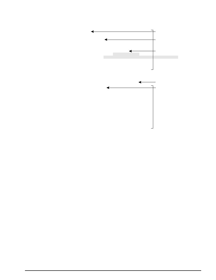
Programmer's Tutorial / Controller Input
9-9
static void disp_sprite()
{
static Sint32 i;
Uint 16 data;
if(!Per_Connect1)return;
data = Smpc_Peripheral[0].data;
for (i=0; i<PAD_NUM;i++){
if((data & pad_asign [i])==0){
slDispSprite((FIXED*)stat[i],
(SPR_ATTR *)(&attr[i],texno),(ANGLE)angz[i];
}
}
}
void main()
{
slInitSystem(TV_320x224,tex_spr,1);
set_sprite(pic_spr,1);
slPrint("Sample program 9.1",slLocate(9,2));
slColRAMMode(CRM16_1024);
slback1ColSet((void*)BACK_COL_ADR,0);
slCharNbg1(COL_TYPE_256,CHAR_SIZE_1x1);
slPageNbg1((void*)NBG1_CEL_ADR,0,PNB_1WORD|CN_12BIT);
slPlaneNbg1(PL_SIZE_1x1);
slMapNbg1((void*)NBG1_MAP_ADR,(void*)NBG1_MAP_ADR,(void*)NBG1_MAP_ADR,
(void*)NBG1_MAP_ADR);
Cel2VRAM(pad_cel,(void*)NBG1_CEL_ADR,483*64);
Map2VRAM(pad_map,(void*)NBG1_MAP_ADR,32,19,1,256);
Pal2CRAM(pad_pal,(void*)NBG1_COL_ADR,256);
slScrPosNbg1(toFIXED(-32.0),toFIXED(-36.0));
slScrAutoDisp(NBG0ON|NBG1ON);
slTVOn();
while(1){
disp_sprite();
slSynch();
}
}
/* display of sprite corresponding to input */
/* device connect check */
/* controller input check */
/* title display */
/* scroll settings */
Note: The lightly shaded portion is defined in "spr_data.c".
Note: The darkly shaded portion is defined in "sega_per.h".
|

9-10
Programmer's Tutorial / Controller Input
Flow Chart 9-1 sample_9_1: Input Test Flow Chart
START
Initialize system
Transfer picture data to
character generator
Set up scrolls
Display scrolls
Get peripheral
data
Execute AND operation
on pad assignments
and peripheral data
Sprite display
Increment assignment
counter
Synchronize
screen
Operation results = 0
Have the
references for all input
mechanisms been
completed?
No
No
Yes
Yes
LOOP
|

Programmer's Tutorial / Controller Input
9-11
Library Functions Used in the Sample Program
Of the library functions used in the sample program, the most important of those which have not
been explained yet in previous chapters are introduced briefly below.
Several other functions that are related to these functions are also introduced briefly.
Sprite functions
These functions are used to display sprites.
Unlike a scroll, a sprite is a type of small unit of graphic data that can be moved and displayed
freely; multiple sprites can be displayed at one time, as well.
Sprites are often used for mobile characters in games that use 3D graphics.
[void slDispSprite (FIXED *pos, ATTR *atrb, ANGLE Zrot);]
This function displays a sprite at the defined position, scale, and display angle.
For the parameters, substitute a four-dimensional array FIXED-type variable pointer that
shows the XYZ coordinate values and the scale value, the starting address of the area where
the sprite data is stored, and the display angle.
As with the library function "slPutPolygon", sorting according to the Z value is performed,
but the current matrix is unaffected.
In addition, if a negative value is substituted for the scale value, then after the scale is calcu-
lated according to the Z value, it is multiplied with the complement of the parameter scale
value and the result is used as the display scale.
For example, if the scale value was specified as "-2.0", and if the sprite is in a position that
would be displayed at 0.5x, it is actually displayed at a scale of 1.0.
[void slPutSprite (FIXED *pos, ATTR atrb, ANGLE Zrot);]
This function calculates the position using the current matrix, and displays the sprite on the
screen with scaling according to the perspective transformation.
For the parameters, substitute a four-dimensional array FIXED-type variable pointer that
shows the XYZ coordinate values and the scale value, the starting address of the area where
the sprite data is stored, and the display angle.
As with "slDispSprite", the sprite is scaled according to the specified scale value, but if a
negative value was substituted, the sprite is reversed top-to-bottom and left-to-right when it
is displayed on the screen.
[void slSetSprite (SPRITE *parms, FIXED Zpos);]
This function sets the sprite control command data to be passed to the hardware into the
transfer list.
For the parameters, substitute the starting address of the area where the sprite data is stored,
and the Z coordinate position.
This function is used only in cases such as when it is desired to set an altered sprite that
cannot be produced with a library function or to set up a window that will affect only special
sprites.
|

9-12
Programmer's Tutorial / Controller Input
Other functions
The two functions introduced here are used for DMA transfers.
In the sample program, the function "slDMACopy" is used to transfer the sprite picture data (a
data transfer from the picture data storage area to the character generator area).
[void slDMACopy (void *src, void *dst, Uint32 cnt);]
This function uses the DMA built into the CPU to make block transfers of data.
For the parameters, substitute the starting address of the area in memory that is the source of
the transfer, the starting address of the area in memory that is the destination of the transfer,
and the size of the bloc transfer (in bytes).
Because this function completes the transfer right after DMA is activated, use the
"slDMAWait" function if you wish to know when the transfer was completed.
[void slDMAWait (void);]
This function waits for completion of a DMA transfer initiated by the library function
"slDMACopy".
The function "slDMACopy" always performs data transfers using the same channel. As a
result, if a previously executed DMA transfer is still in progress, subsequent data transfers
are initiated only after waiting for the previous transfer to be completed.
Fig. 9-8 "slDMAXCopy" Parameter Substitution Values (mode)
Destination
Increment
Decrement
Fixed
Source
Increment
Sinc_Dinc_Byte
Sinc_Ddec_Byte
Sinc_Dfix_Byte
Decrement
Sdec_Dinc_Byte
Not allowed
Sdec_Dfix_Byte
Fixed
Sfix_Dinc_Byte
Sfix_Ddec_Byte
Not allowed
Note: The above values are defined in "sl_def.h".
Note: The above values assume the unit of transfer is "byte". "Word" and "long" can also be specified as
the unit of transfer.
Supplement. SGL Library Functions Covered in this Chapter
The functions listed in the following table were explained in this chapter.
Table 9-3 SGL Library Functions Covered in this Chapter
Function type
Function name
Parameters
Function
void
slDispSprite
FIXED *pos, ATTR *atrb,
Display sprite at specified position, scale, and
ANGLE Zrot
display angle
void
slPutSprite
FIXED *pos, ATTR *atrb,
Display sprite with perspective transformation
ANGLE Zrot
void
slSetSprite
SPRITE *parms, FIXED Zpos
Set sprite data in hardware
void
slDMACopy
void *src, void *dst, Uint32 cnt
Perform DMA transfer from A to B, for C bytes
(identical bus transfer possible)
void
slDMAWait
void
Wait until DMA transfer is completed
|

Event Control
This chapter explains event structures and specifically how to
use the event management functions. By using the event
concept, it is possible to describe a program as a combination of
program events (each of the elements within the program),
making it very easy to understand the flow of the program as a
whole.
In addition, because program events can be shared, program
simplification is possible.
Programmer's Tutorial
10
|

10-2
Programmer's Tutorial / Event Control
Structure of Events
Event processing
Event processing consists of labeling a group of functions registered within the program listing
as an "event" and then executing a list of consecutive events in order.
By using event processing, it becomes possible to process complex groups of consecutively
executed functions as a simple list of labels. In addition, the execution sequence can be easily
changed around by manipulating the labels registered as events.
This approach makes it possible to grasp the flow of a program as a whole; in addition, events
can be shared, making program simplification possible.
Fig 10-1 The Event Concept
slInitEvent();
slSetEvent((void*)game_demo);
slSetEvent((void*)game_play);
slSetEvent((void*)game_over);
slExecuteEvent();
void game_demo(EVENT*evptr){
...
}
void game_play(EVENT*evptr){
...
}
void game_over(EVENT*evptr){
...
}
/* event initialization */
/* event registration */
/* event execution */
/* event 1 (game_demo) */
/* event 2 (game_play) */
/* event 3 (game_over) */
/* omitted */
/* omitted */
Event list
game_demo
game_play
game_over
Executed in
sequence of
registration
The execution sequence can easily be changed
(additions, insertions, deletions) by using the
event management function.
The function groups registered as events and the event execution sequence are processed in
event management areas called "event structures" allocated in a RAM area used for events.
In the SGL, the event execution sequence is called the "event list."
|

Programmer's Tutorial / Event Control
10-3
Event structures
Events are defined as EVENT structures (size: 128 bytes) in the event RAM area (size: 8K); one
EVENT structure consists of 128 bytes, and a maximum of 64 EVENT structures can be de-
fined in this RAM area.
The configuration of an EVENT structure is shown in Fig 10-2.
Fig 10-2 EVENT Structure
EVENT structure 1
EVENT structure 2
EVENT structure 3
user
(112byte)
(4byte)
(4byte)
(4byte)
(4byte)
*exad()
*before
*next
*work
EVENT structure 62
EVENT structure 62
EVENT structure 62
Event RAM area
128byte
64
=819byte
=8kbyte
×
128byte
a) Event RAM area
b) Event structure
*work: Work structure address; NULL if
work structure is not used
*next:
Execution address of next event;
NULL if last event
*before: Execution address of previous
event; NULL if first event
*exad(): Event execution address
user:
Area used for storing variables used
by the event
Each EVENT structure consists of the following members:
*work:
Starting address of the work structure used to extend the user area
*next:
Starting address of the event to be executed next
*before: Starting address of the event that was executed last
*exad(): Starting address where the functions that are to be executed as the event are stored
user[]:
User area used for storing variables used by the functions registered in the event;
the user
area can be extended by using a work structure, etc.
If there is no corresponding address for "*work", "*next", or "*before", NULL is substituted.
If the user is going to use the user area within the EVENT structure, it is useful to "cast" the
user area as a structure defined for users.
Although the user area in one EVENT structure consists of 112 bytes, the work structure, etc.,
can be used to extend the user area if desired. For details on how to extend the user area, refer
to the section on user area extension.
|

10-4
Programmer's Tutorial / Event Control
Event lists
Each event defined as an EVENT structure within the event RAM area forms a list of events in
the sequence they are to be executed in.
The list is tied together by the members "*next" and "*before" reserved in the EVENT struc-
ture. The series of events to be executed is called an "event list."
The events executed in sequence within the event list do not have to be stored in sequence in the
event RAM; as long as the events are linked by the "*next" and "*before" pointers, the events
will be executed in the proper sequence.
Fig 10-3 Event List Structure
EventTop
EventLast
EventNow
EventNow
user[]
EVENT structure 1
*exad()
*before = NULL
*next
*work = NULL
user[]
EVENT structure 2
*exad()
*before
*next
*work
*next
*next = NULL
user[]
user[]
Work structure 1
Work structure 2
user[]
EVENT structure 3
*exad()
*before
*next = NULL
*work = NULL
EventTop:
Starting address of top event
EventLast:
Starting address of last event
EventNow:
Starting address of event currently being executed
The "next" address from the previous event is
substituted.
*next:
Starting address of next event or work structure
*before:
Starting address of previous event
*work:
Starting address of work structure to be used
Note:
If the event or work address in question does not
exist: NULL
The system puts the starting address of the EVENT structure registered at the start of the event
list into the variable "EventTop"; when the system executes the event list, it executes the events
in sequence, starting with the event specified by "EventTop".
The value of the "*next" pointer in the EVENT structure of the event that was just executed is
passed to the "EventNow" variable, and the system next begins executing the EVENT structure
that starts at the address indicated by "EventNow". The system continues to execute the events
in sequence according to "EventNow", and then terminates event execution processing when
the value of "*next" is null, indicating that there are no more subsequent events. The
"EventLast" variable points to the starting address of the EVENT structure registered last in the
list, and is used when adding or registering events. The "EventLast" variable is changed only
by the execution of the following library functions: "slSetEvent", "slSetEventNext", and
"slCloseEvent". "*before" is used when inserting, registering, or deleting events.
|

Programmer's Tutorial / Event Control
10-5
Event Processing Using SGL Functions
This section explains actual event processing using the SGL library functions.
Event initialization
In order to use event processing in the SGL, it is necessary to first initialize the event-related
buffers and the event list.
Note that if event processing is used without executing event initialization, coordination with
the uninitialized buffers and event list will not be possible, with the result in the worst case
being that the CPU stops operating. (For details, refer to "Cautions Concerning Event Process-
ing.")
In the SGL, use the library function "slInitEvent" to execute event initialization.
[void slInitEvent (void);]
This function performs all initializations (event list and buffer initializations, etc.) involved
in event processing.
Creating an Event List
In order to perform event processing, it is necessary to register events in the event list in the
order that they are to be executed in.
Events are added to an event list as shown in Fig 10-4 below by the event registration library
function "slSetEvent".
The registered events are appended in sequence at the end of the event list. The event execution
library function "slExecuteEvent" is used to initiate execution of the event list, starting from the
top of the list.
Fig 10-4 Creating an Event List
Register event A
Event A
Event A
Event A
Event B
Event B
Event C
Register event B
Register event C
Event list
Use the library function "slSetEvent" to register events.
|

10-6
Programmer's Tutorial / Event Control
[EVENT *slSetEvent (void (*func)();]
This function allocates an EVENT structure (size: 128 bytes) in the event RAM area, and
adds/registers new events at the end of the event list. For the parameter, substitute the
execution address for the event being registered. As a return value, this function returns the
starting address of the EVENT structure that was registered. If event registration failed, the
null value is returned.
For details on event format and structure, refer to the next page.
Event format
The group of functions registered as events must have the format shown in Fig 10-5:
Fig 10-5 Event Format
void function_name(EVENT *evptr){execute_contents}
·
·
Event format
Event execution contents
Event name
Starting address of EVENT structure
The events that are to be registered or executed are managed through the EVENT structure.
The execution addresses of the registered events and the structures for the variables used within
the events are stored in the EVENT structure; these two elements are used to manage the events.
Fig 10-6 Structure of an Event
slSetEvent((void*)int_cube);
slExecuteEvent();
typedef struct cube{ FIXED pos[xyz];
ANGLE ang[xyz];
|
Sint16
unset_count;
Sint16
unset-i;
}CUBE;
void int_cube(EVENT*evptr)
[
CUBE
*cubeptr;
cubeptr=(CUBE*)evptr->user;
cubeptr->pos[x]=pos_x;
|
cubeptr->unset_count=0;
disp-cube(evptr);
}
/* event registration */
/* event execution */
/* cube structure definition */
/* event (init_cube) */
/* cast user area in CUBE structure */
/* change variable (cube structure) */
/* functions called in the event */
/* omitted */
/* omitted */
EVENT structure
user[]
*exad()
*before
*next
*work
pos[xyz]
unset_count
ang[xyz]
unset_i
Event execution address
(void*)init_cube
Store
Store
CUBE structure
·
·
·
·
Functions registered as events are controlled through EVENT
structures.
The execution address of a registered event is stored in the
member "exad()" and the structure used by the event is stored
in the member "user[]".
Although structures are used for variables within events, be
careful not to let the structure exceed the size of the user area
(112 bytes).
To use a larger number of variables, extend the user area by
utilizing the work structure, etc., and partition the structure
itself for storage.
Structures for variables within an event
When a variety of variables are used within an event, it is necessary to define that
variable group as a structure.
The defined event variable structure is stored in the user area (size: 112 bytes) in the
EVENT structure when the event is registered (the user must perform the storage
task); the event variable structure can thereafter be used immediately.
|

Programmer's Tutorial / Event Control
10-7
Accordingly, the event variable structure cannot be set up so that it exceeds the size
(112 bytes) of the user area in which the structure is stored.
However, use even more variables, extend the user area by utilizing the work structure,
etc., and partition and store the event variable structure so that it does not exceed the
size of the user area. (For details on how to extend the user area, refer to "Extending
the User Area.")
Event execution
The events registered in the event list are executed in sequence by the event management
functions. Use the library function "slExecuteEvent" to execute the events.
For example, after the library function "slSetEvent" is used to register event A, event B, and
event C in the event list in that sequence, each event is executed according to the event list in
the sequence shown in the following diagram.
Fig 10-7 Event Execution
Event A
Event B
Event C
Event list
Execute in sequence, starting from event A
[void slExecuteEvent (void);]
This function executes the events registered in the event list in the sequence that they have in
the list.
|

10-8
Programmer's Tutorial / Event Control
Changing the Event List
Adding events
Events can be added to the events registered in the event list.
Events are added at the end of the event list.
The same library function, "slSetEvent", that was used to register events is also used to add
events.
Fig 10-8 Adding Events
Event A
Event A
Event B
Event B
Event C
Event C
Event list
Event list
Add
[EVENT *slSetEvent (void (*func)());]
This function allocates an EVENT structure (size: 128 bytes) in the event RAM area, and
adds/registers new events at the end of the event list. For the parameter, substitute the
execution address for the event being registered. As a return value, this function returns the
starting address of the EVENT structure that was registered. If event registration failed, the
null value is returned.
Event insertion
This function inserts an event among the events registered in the event list.
The new event is inserted right after the specified event.
The library function "slSetEventNext" is used to insert events.
Fig 10-9 Event Insertion
Event A
Event A
Event B
Event C
Event A
Event C
Event B
Event list
Event list
after
Insert
[EVENT *slSetEventNext (EVENT *evptr, void (*func)());]
This function allocates an EVENT structure (size: 128 bytes) in the event RAM area, and
inserts/registers new events in the middle of the event list. For the parameter, substitute the
starting address of the EVENT structure immediately before the point where the new event
is to be inserted, and the execution address for the event being inserted/registered. As a
return value, this function returns the starting address of the EVENT structure that was
registered. If event registration failed, the null value is returned.
|

Programmer's Tutorial / Event Control
10-9
Event deletion
Events registered in an event list can be deleted from the list. Use the library function
"slCloseEvent" to delete the event.
Fig 10-10 Event Deletion
Event A
Event A
Event C
Event B
Event B
Event C
Event list
Event list
Delete
[void slCloseEvent (EVENT *evptr);]
This function deletes the event specified by the parameter from the event list.
At the same time, if the member "work" of the specified event is not "NULL", all of the
associated work is returned to the system as a work list.
For the parameter, substitute the starting address of the EVENT structure to be deleted.
In addition, this function "slCloseEvent" does not check to make sure that the area being
returned is an EVENT structure. Therefore, if you accidentally return an extended user area
back to the system, this function will not detect the error.
If this type of mistake occurs, various problems can arise, and in the worst case the CPU will
stop operating. (For details, refer to "Cautions Concerning Event Processing.")
Changing the event list during event execution
If any type of attempt is made to change an event list that contains registered events and is in
the process of being executed (including changes among the events in the event list, etc.) the
changed event is affected as shown in the following diagram.
Fig 10-11 Changing the Event List During Execution
Event A
Inserted event 1
Inserted event 2
Added event
Event B
Event C
Event list
Event D
Event E
Event F
Event currently being executed
Inserted event 1:
Executed the next time the event list is
executed
Inserted event 2:
Executed this time after event D
Added event:
Executed this time after event F
|

10-10
Programmer's Tutorial / Event Control
Changes to the event list that are before the event currently being executed (in the part of the list
that has already been executed) apply the next time the event list is executed.
Changes to the event list that are after the event currently being executed (in the part of the list
that has not yet been executed) are executed according to the sequence of the newly changed
event list during this execution of the event list.
All changes, whether additions, insertions, or deletions, are applied in the same way.
|

Programmer's Tutorial / Event Control
10-11
Extending the User Area
When describing a program by using event processing, there may be times when the variable
group (structure) used by a function being executed as an event will not fit within the user area
(112 bytes) of the event.
In these circumstances, it is possible in the SGL to extend the user area.
There are two methods for extending the user area: one is to use the work area as a dedicated
extension area, and the other is to allocate an extension area the same size as an EVENT struc-
ture within the event RAM area.
Extending a user area with a work area
In the SGL, it is possible to extend the user area in an EVENT structure by using a dedicated
user area extension area called the "work area."
A work area is defined as a WORK structure (size: 64 bytes) within the working RAM area; up
to 256 work areas can be used.
One work area can increase the size of the user area by 60 bytes. The remaining four bytes of
the WORK structure are used for specifying the address of a linked WORK structure.
Fig 10-12 WORK Structure
WORK structure 1
WORK structure 2
WORK structure 3
user[]
(60byte)
(4byte)
*next
WORK structure 254
WORK structure 255
WORK structure 256
Working RAM area
64byte
256
=16384byte
=16kbyte
×
64byte
a) Working RAM area
b) WORK structure
*next:
Starting address of a linked WORK
structure
user[]: Area used for storing variables
by the event
The WORK structure members are as follows:
*next:Starting address of a WORK structure linked in a chain; if there is no WORK structure
that follows in a chain, NULL.
user[]:Extended user area (size: 60 bytes)
A work area allocated as a WORK structure can be linked in chain fashion by substituting the
starting address for the WORK structure in the "*work" member of the EVENT structure.
In addition, by allocating another work area within a WORK structure, it is possible to further
extend the user area.
In this case, by substituting the starting address of the next WORK structure to be chained in the
"*next" member of the previous WORK structure, it is possible to chain together WORK
structures.
|

10-12
Programmer's Tutorial / Event Control
If there is no WORK structure that follows in the chain, NULL is substituted for the "*next"
member of the last WORK structure.
Fig 10-13 Work Area Chaining
user
user[]
user[]
user[]
*exad()
*before
*next
*next
*next
*next = NULL
*work
EVENT structure
WORK structure 1
WORK structure 2
WORK structure 3
A user area extended through work areas is chained together through
the addresses specified in the "*work" member of the EVENT structure
and the "*next" member of the WORK structures.
To use work areas in the SGL, use the library functions "slGetWork" and "slReturnWork".
[WORK *slGetWork (void);]
This function allocates a WORK structure (size: 64 bytes) in the working RAM area.
As a return value, this function returns the starting address of the WORK structure that was
allocated. If area allocation failed, the null value is returned.
[void slReturnWork (WORK *wkptr);]
This function returns/releases the work area specified by the parameter. For the parameter,
specify the WORK structure address of the work area being returned. In addition, if return-
ing/releasing part of a chain of work areas to the system, adjust the chain structure of the
remaining work areas so that the chain structure is correct. If adjustments are not made, it
will be impossible to coordinate the chain structure and work processing, with the possible
result that the CPU will stop operating. (For details, refer to the next section.)
Operation of chained WORK structures after the release of an EVENT structure
Work areas do not necessarily have to be chained together by the "*work" and "*next"
members; it is also possible to store the starting address of a linked WORK structure in
the user area. Work areas chained together by the "*work" and "*next" members are
returned/released to the system simultaneously if the associated event is released, but
WORK structures linked through the user area are not released if the event is released.
Therefore, when an event is released, it is necessary to use the library function
"slReturnWork" to return/release to the system those WORK structures that were
linked through the user area.
|

Programmer's Tutorial / Event Control
10-13
Extending the user area with event areas
If a WORK structure (size: 60 bytes) does not provide enough space for one user area to be
extended it is possible to allocate a user area the same size as an EVENT structure (size: 128
bytes) in the event RAM area.
However because an area originally allocated for the use of an event is being used as a user
area, the maximum number of events that can be registered decreases accordingly.
Fig 10-14 Using the Event RAM Area to Extend a User Area
EVENT structure 1
EVENT structure 2
EVENT structure 3
user
user
Extended user area
Extended user area
(112byte)
(128byte)
(4byte)
(4byte)
(4byte)
(4byte)
*work
*before
*next
*exad()
EVENT structure 62
Extended user area
EVENT structure 63
Event RAM area
EVENT structure 1
Used as a user area, but decreases the maximum number of events that can be registered
In the SGL, when the user area of an EVENT structure is to be extended by using the event
RAM area, use the library functions "slGetEvent" and "slReturnEvent".
"slGetEvent" is used to allocate the user area, and "slReturnEvent" is used to release the user
area.
[EVENT *slGetEvent (void);]
This function allocates a user area in event RAM the same size as an event (size 128 bytes).
Because an area originally allocated for the use of an EVENT structure is being used as a
user area, the maximum number of events that can be registered decreases accordingly.
As a return value, this function returns the starting address of the RAM area that was allo-
cated. If area allocation failed, the null value is returned.
[void slReturnEvent (EVENT *evptr);]
This function returns/releases the event RAM area specified by the parameter back to the
system.
For the parameter, substitute the starting address of the RAM area being returned.
In addition, this function "slReturnEvent" does not check to make sure that the area being
returned is an extended user area. Therefore, if you accidentally return an EVENT structure
that is registered as an event back to the system, this function will not detect the error.
If this type of mistake occurs, various problems can arise, and in the worst case the CPU will
stop operating. (For details, refer to "Cautions Concerning Event Processing.")
|

10-14
Programmer's Tutorial / Event Control
Cautions Concerning Event Processing
In event processing, particular caution is required when returning/releasing various areas back
to the system. This is because during the release/return operation, the function being used does
not check to make sure that the area specified by the parameter is an area of the type for which
the function is intended.
For example, if an attempt is made to return/release an extended user area with the library
function "slReturnEvent", but an area registered as a normal event is accidentally returned/
released, the problems like the following can arise, with the CPU ceasing to operate in the worst
case.
1) Return of area:
The specified EVENT structure is returned to the system by the function "slReturnEvent".
2) Event list
Because the event structure was not released as an event, it continues to exist in the event
list.
3) New event registration
Because the area is free as far as the system is concerned, the area can be used by the func-
tion "slSetEvent", etc.
4) Chain structure conflict
Event though it is registered in the event list, the area is regarded to be free, so the contents
of the EVENT structure are overwritten, which can create problems in chained structures.
5) CPU halt
Because the chain structure cannot be coordinated, in the worst case the CPU will stop
operating.
Fig 10-15 Incorrect Event Operations
user[]
user[]
user[]
*work
*work
*work
*before = NULL
*before
*before
*next
*next
*next = NULL
*exad()
*exad()
*exad()
EVENT structure 1
EVENT structure 2
EVENT structure 3
user[]
user[]
user[]
*work
*work
*work
*before = NULL
*before
*before
*next
*next = NULL
*next
*exad()
*exad()
*exad()
EVENT structure 1
EVENT structure 2
EVENT structure 3
EventTop
EventTop
EventLast
EventLast
Incorrect event operation
a) Normal chain structure
b) Disrupted chain structure
1) EVENT structure 2 is released
by the function "slReturnEvent".
2) The event list is not changed.
3) The function "slSetEvent" is executed.
4) EVENT structure 2 is added/registered
as a new, different event.
5) The chain structure is disrupted, and
future event operations could result in
the CPU ceasing to operate.
|

Programmer's Tutorial / Event Control
10-15
Flow of Event Processing
The following flow chart is a broad summary of the flow of event processing. In event process-
ing, it is also possible to extend the user area within the event being executed when necessary
and to use variables in structures.
Flow Chart 10-1 Flow of Event Processing
START
Initialize events
"slInitEvent"
Register events
"slSetEvent"
Add events
"slSetEvent"
Execute events
"slExecuteEvent"
Insert events
"slSetEventNext"
Synchronize screen
"slSynch"
Delete events
"slCloseEvent"
LOOP
|

10-16
Programmer's Tutorial / Event Control
Example of Event Usage
The following sample program, "sample_10" (List 10-1 and List 10-2), is an example of pro-
gramming that actually uses event processing.
In the program, events are used to control/execute the display/non-display of a cube.
The program basically consists of two parts: "main.c" (List 10-1) initializes the system and
executes the events, and "sample.c" (List 10-2) initializes the events, defines the contents of the
events, and registers the events.
List 10-1 sample_10: Event Processing (main.c)
/*----------------------------------------------*/
/*
Event Control
*/
/*----------------------------------------------*/
#include "sgl.h"
void set_event();
void main()
{
slInitSystem(TV_320X224,NULL,1);
slPrint("Sample program 10",slLocate(9,2));
set_event();
while(-1)
{
slExecuteEvent();
slSynch();
}
}
/*----------------------------------------------*/
/* include file containing various settings */
/* system initialization */
/* title display */
/* event list creation */
/* event execution */
/* scan line synchronization */
Note: The lightly shaded portion is defined in "sgl.h" and "sl_def.h".
Note: The darkly shaded portion is defined in "sample.c".
Flow Chart 10-2 sample_10: Main Loop
START
Initialize system
Create event list
"set_event"
Execute events
registered in event list
Synchronize
screen
|

Programmer's Tutorial / Event Control
10-17
The following listing from sample_10_1 shows the portion where events are registered and the
contents of the events are defined.
In the user-defined function "disp_cube", the contents of the event list are changed (added/
deleted).
List 10-2 sample_10: Event Processing (sample.c)
#include
"sgl.h"
extem PDATA PD_CUBE;
#define
POS_X
toFIXED(0.0)
#define
POS_X_UP
200.0
#define
POS_Y
toFIXED(20.0)
#define
POS_Z
toFIXED(270.0)
#define
POS_Z_UP
50.0
#define
SET_COUNT
500
static void init_cube2(EVENT*);
typedef struct cube{
FIXEDpos[XYZ];
ANGLE
ang[XYZ];
ANGLE
angx,angz;
ANGLE
anx_up,angz_up;
PDATA*poly;
Sint16 set_count,set_i;
Sint16 unset_count,unset_i;
}CUBE;
static void disp_cube(EVENT*evptr)
{
CUBE *cubeptr;
cubeptr=(CUBE*)evptr->user;
slPushMatrix();
{
slTranslate(cubeptr->pos[X],cubeptr->pos[Y],cubeptr->pos[Z];
cubeptr->pos[X]=POS_X+POS_X_UP*slSin(cubeptr->angx);
cubeptr->pos[Y]=cubeptr->pos[Y];
cubeptr->pos[Z]=POS_Z+POS_Z_UP*slCos(cubeptr->angz);
cubeptr->angx+=cubeptr->angx_up;
cubeptr->angz+=cubeptr->angz_up;
slRotY(cubeptr->ang[Y];
slRotX(cubeptr->ang[X];
slRotZ(cubeptr->ang[Z];
cubeptr->ang[X]+=DEGtoANG(5.0);
cubeptr->ang[Y]+=DEGtoANG(5.0);
cubeptr->ang[Z]+=DEGtoANG(5.0);
slPutPolygon(cubeptr->poly);
}
slPopMatrix();
cubeptr->set_count-=cubeptr->set_i;
if(cubeptr->set_count<0){
slSetEvent((void*)init_cube2);
cubeptr->set_count=SET_COUNT;
}
cubeptr->unset_count-=cubeptr->unset_i;
if(cubeptr->unset_count<0)slCloseEvent(evptr);
}
/* include file containing various settings */
/* CUBE structure definition */
/* polygon drawing routine */
/* CUBE structure modification */
/* polygon drawing start */
/* event list change routine */
/* event addition (init_cube2) */
/* event deletion (init_cube2) */
(continued on next page)
|

10-18
Programmer's Tutorial / Event Control
static void init_cubel(EVENT*evptr)
{
CUBE *cubeptr;
cubeptr=(CUBE*)evptr->user;
cubeptr->pos[X]=POS_X;
cubeptr->pos[Y]=POS_Y;
cubeptr->pos[Z]=POS_Z;
cubeptr->ang[X]=cubeptr->ang[Y]=cubeptr->pos[Z]=DEGtoANG(0.0);
cubeptr->angx=cubeptr->angz=DEGtoANG(0.0);
cubeptr->angx up=cubeptr->angz_up=DEGtoANG(0.0);
cubeptr->set_count=SET_COUNT;
cubeptr->set_i=1;
cubeptr->unset_count=0;
cubeptr->unset i=0;
cubeptr->poly=&PD_CUBE;
evptr->exad=(void*)disp_cube;
disp_cube(evptr);
}
static void init_cube2(EVENT *evptr)
{
CUBE *cubeptr;
cubeptr=(CUBE*)evptr->user;
cubeptr->pos[X]=POS_X;
cubeptr->pos[Y]=POS_Y-toFIXED(50);
cubeptr->pos[Z]=POS_Z+POS_Z_UP;
cubeptr->ang[X]=cubeptr->ang[Y]->cubeptr->ang[Z]=DEGtoANG(0.0);
cubeptr->angx=cubeptr->angz=DEGtoANG(0.0);
cubeptr->angx_up=cubeptr->angz_up=DEGtoANG(3.0)*(-1);
cubeptr->set_count=0;
cubeptr->set_i=0;
cubeptr->unset_count=SET_COUNT/2;
cubeptr->unset_i=1;
cubeptr->poly=&PD_CUBE:
evptr->exad=(void*)disp_CUBE;
disp_cube(evptr);
}
staric Void init_cube3(EVENT*evptr)
{
CUBE *cubetr;
cubeptr=(CUBE*)evptr->user;
cubeptr->pos[X]=POS_X;
cubeptr->pos[Y]=POS_Y-toFIXED(50);
cubeptr->pos[Z]=POS_Z+POS_Z_UP;
cubeptr->ang[X]=cubeptr->ang[Y]->cubeptr->ang[Z]=DEGtoANG(0.0);
cubeptr->angx=cubeptr->angz=DEGtoANG(0.0);
cubeptr->angx_up=cubeptr->angz_up=DEGtoANG(3.0);
cubeptr->set_count=0;
cubeptr->set_i=0;
cubeptr->unset_count=0;
cubeptr->unset_i=0;
cubeptr->poly=&PD_CUBE:
evptr->exad=(void*)disp_cube;
disp_cube(evptr);
}
void*event_tbl[]={
init_cube1,
init_cube2,
init_cube3
};
void set_event()
{
EVENT*evptr;
void **exptr;
Uint16 cnt
slInitEvent();
for(exptr=event_tbl,cnt=sizeof(event_tbl)/sizeof(void*);cnt-->0;){
evptr=slSetEvent(*exptr++);
}
}
/* event 1 (init_cube1) */
/* event 1 execution contents */
/* CUBE1 display */
/* event 2 (init_cube1) */
/* event 2 execution contents */
/* CUBE2 display */
/* event 3 (init_cube1) */
/* event 3 execution contents */
/* CUBE3 display */
/* event registration table */
/* event initialization */
/* set events according to event table */
|

Programmer's Tutorial / Event Control
10-19
The following flow chart is a summary of the event execution contents.
The event execution contents differ the first time through the loop compared to the second and
subsequent times through the loop. In the flow chart, the left side indicates the event execution
contents the first time through the loop, and the right side indicates the event execution contents
the second and subsequent times through the loop.
Flow Chart 10-3 sample_10_1: Event Execution Contents
Event execution
contents (first time)
Event execution
contents (second and
subsequent times)
Set initial angle
of object
Place object
Set initial position
of object
Temporarily allocate
operation matrix (push)
Call operation
matrix
Decrement
registration counter
Register event
in event list
Release event
from event list
Set registration
counter
End
Decrement
release counter
Set counter for event
registration ad release
Correct object
position
Change event list
Correct object
display angle
Draw object
Register polygon
data
Set object
display angle
Is registration
counter < 0?
Is release
counter < 0?
|

10-20
Programmer's Tutorial / Event Control
Supplement. SGL Library Functions Covered in this Chapter
The functions listed in the following table were explained in this chapter.
Table 10-1 SGL Library Functions Covered in this Chapter
Function type
Function name
Parameters
Function
void
slInitEvent
void
Initialize events
EVENT
*slSetEvent
void (*func)()
Register/add an event to the event list
void
slExecuteEvent
void
Execute events registered in the event list in
sequence
EVENT
*slSetEventNext
EVENT *evptr,
Insert/register a new event right after the
void (*func)()
specified registered event
void
slcloseEvent
EVENT *evptr
Delete an event from the event list and return
release the associated work areas to the system
WORK
*slGetWord
void
Allocate a work area
void
slReturnWork
void
Return/release a work area
EVENT
*slGetEvent
void
Allocate a RAM area the same size as an event in
the event RAM area
void
slReturnEvent
EVENT *evptr
Return/release to the system an area that was
allocated by using "slGetEvent"
|

Mathematical Operation
Functions
This chapter introduces the various mathematical operation
functions supported in the SGL.
Programmer's Tutorial
11
|

11-2
Programmer's Tutorial / Mathematical Operation Functions
General Mathematical Operation Functions
The following are the general mathematical operation functions.
[FIXED slDivFX (FIXED a, FIXED b);]
This function divides parameter "b" by parameter "a".
[FIXED slMulFX (FIXED a, FIXED b);]
This function multiplies parameter "a" by parameter "b".
[FIXED slSquartFX (FIXED sqrtfx);]
This function returns the square root of an unsigned fixed-point (FIXED-type) value.
[Uint32 slSquart (Uint32 sqrt);]
This function returns the square root of an unsigned integer value.
|

Programmer's Tutorial / Mathematical Operation Functions
11-3
Trigonometric Functions
The trigonometric operation functions are listed below.
[FIXED slSin (ANGLE angs);]
This function returns the sine value of the specified angle (ANGLE-type).
[FIXED slCos (ANGLE angs);]
This function returns the cosine value of the specified angle (ANGLE-type).
[FIXED slTan (ANGLE angs);]
This function returns the tangent value of the specified angle (ANGLE-type).
Fig 11-1 Model of Trigonometric Functions
r
ty
tx
Y
X
sin
= ty/r = slSin( )
cos
= tx/r = slCos ( )
Tan
= ty/tx = slTan( )
[ANGLE slAtan (FIXED tx, FIXED ty);]
This function returns the angle of the specified direction.
Fig 11-2 Model of "slAtan"
ty
tx
Y
X
Tan
= ty/tx ;
= tan ty/tx = slAtan(tx,ty) ;
-1
|

11-4
Programmer's Tutorial / Mathematical Operation Functions
Special Operation Functions
The special operation functions are listed below.
[FIXED slCalcPoint (FIXED cx, FIXED cy, FIXED cz, FIXED *ret);]
This function multiplies the specified point by the current matrix and substitutes the result in the
parameter "ret".
[FIXED slInnerProduct (VECTOR a, VECTOR b);]
This function calculates the vector inner product between the specified parameters.
The value shown in Fig 11-3 is returned.
Fig 11-3 Value Returned by the Vector Inner Product Operation
A(X1,Y1,Z1)*B(X2,Y2,Z2) = X1*X2+Y1*Y2+Z1*Z2
= Return Value;
·
·
Value Returned by the Vector Inner Product Operation
[Uint32 slDec2Hex (Uint32 val);]
This function converts a value expressed in BCD code to hexadecimal code.
[Uint32 slHex2Dec (Uint32 val);]
This function converts a value expressed in hexadecimal code to BCD code.
[Uint16 slAng2Hex (ANGLE ang);]
This function converts an angle value expressed in ANGLE code to hexadecimal code. The
converted value that is returned ranges from 0 to 359.
[Uint16 slAng2Dec (ANGLE ang);]
This function converts an angle value expressed in ANGLE code to BCD code. The con-
verted value that is returned ranges from 0 to 359.
[FIXED slAng2FX (ANGLE ang);]
This function converts an angle value expressed in FIXED code to binary code. The con-
verted value that is returned ranges from 0 to 359.
Table 11-1 Examples of value notation using each notation method
Decimal
BCD
Hexadecimal
Notation
92
0x92
0x5cH
|

Programmer's Tutorial / Mathematical Operation Functions
11-5
Supplement. SGL Library Functions Covered in this Chapter
The functions listed in the following table were explained in this chapter.
Table 11-2 SGL Library Functions Covered in this Chapter
Function type
Function name
Parameters
Function
FIXED
slDivFX
FIXED a, FIXED b
Division (B/A)
FIXED
slMulFX
FIXED a, FIXED b
Multiplication (A * B)
FIXED
slSquartFX
FIXED sqrtfx
Return square root of unsigned fixed-point value
Uint32
slSquart
Uint32 sqrt
Return square root of unsigned integer value
FIXED
slSin
ANGLE angs
Return sine value of specified angle
FIXED
slCos
ANGLE angc
Return cosine value of specified angle
FIXED
slTan
ANGLE angt
Return tangent value of specified angle
ANGLE
slAtan
FIXED tx, FIXED ty
Return angle of specified direction
FIXED
slCalcPoint
FIXED zx, cy, cz,
Multiply specified point by the current matrix
FIXED *ret
FIXED
slInnerProduct
VECTOR a, VECTOR b
Calculate vector inner product
Uint32
slDec2Hex
Uint32 val
Convert from BCD code to Hexadecimal code
Uint32
slHex2Dec
Uint32 val
Convert from Hexadecimal code to BCD code
Uint16
slAng2Hex
ANGLE ang
Convert from ANGLE code to Hexadecimal code
Uint16
slAng2Dec
ANGLE ang
Convert from ANGLE code to BCD code
FIXED
slAng2FX
ANGLE ang
Convert from ANGLE code to FIXED code
|

CD-ROM Library
This chapter explains how to use the CD-ROM library to access
CD-ROM. The CD-ROM library makes it possible to load
programs and data from CD-ROM and also to play music.
This chapter also includes the function reference for the CD-
ROM library.
Programmer's Tutorial
12
|

12-2
Programmer's Tutorial / CD-ROM Library
The CD-ROM Library
The SGL includes functions for accessing CD-ROM and virtual CDs.
These functions can be used to implement the following functions:
·
Loading programs and data from CD-ROM
·
Loading data according to the CD-ROM XA standard
·
Playing back music using CDDA files
Note: The CD-ROM library functions are not listed in the separate Function Refer-
ence. Instead, they are included at the end of this chapter.
For details on writing to a CD-ROM, refer to the reference Transferring Data, chapter 3, "Writ-
ing CD-ROM."
|

Programmer's Tutorial / CD-ROM Library
12-3
Accessing CD-ROM
The flow of operations for loading data from a CD-ROM is described below.
Fig 12-1 CD-ROM Access Flow Chart
Initialize CD library
slCdInit()
slCdOpen()
slCdLoadFile()
slCdGetStatus()
Start
End
Open file
Request load
Get status
Loading
completed?
No
Yes
Because CD-ROM access entails mechanical operations, the data is not loaded into memory at
the instant that the load request is made. In addition, in comparison with the operational speed
of the CPU, the speed at which the data is loaded from the CD-ROM is extremely slow. In
order to permit the execution of operations aside from the CD-ROM access during this wait, the
SGL supports a method in which the loading status is monitored during CD-ROM access.
Logical Structure of CD-ROM
CD-ROM consists of units called "sectors." Although sectors generally contain 2048 bytes
(FORM1), in cases such as music where a few misread bits will not cause problems and a high
transfer capacity is desired, it is possible to put 2324 bytes (FORM2) into each sector. Each
sector within a file contains a subheader consisting of the channel number, submode, and coding
information.
|

12-4
Programmer's Tutorial / CD-ROM Library
Fig 12-2 Sector Structure
Data (2048 bytes)
Data (2324 bytes)
FORM1
FORM2
Subheader
Subheader
Error correction
information
The SGL includes a function that classifies data according to the subheader. This information is
called a "key" in the SGL. Each bit of the submode and coding information is significant, and
in the SGL, only those sectors in which the specified bits are set to "1" are selected and loaded.
Loading files
Use the functions "slCdOpen", "slCdLoadFile", and "slCdGetStatus" to load files.
CDHN slCdOpen (Sint8 *pathname, CDKEY key []);]
This function specifies the file to be loaded.
"key" specifies the type of sector to be loaded. Multiple sector types can be specified. After
all sector types have been specified, specify "CDKEY_TERM" for the last channel number.
Once the file is opened correctly, a file handle other than "NULL" is returned.
If the maximum number of keys for an open file reaches 24 or more, the open operation
fails. The open file is closed automatically when the loading operation is interrupted or
completed.
[Sint32 slCdLoadFile (CDHN cdhn, CDBUF buf []);]
This function specifies the area into which the file is to be loaded.
The sequence of "buf" corresponds to the sequence of "key" in the function "slCdOpen".
When copying the CD-ROM data to the work RAM, make the following specifications:
buf[i].type = CDBUF_COPY;
buf[i].trans.copy.addr = loading area address;
buf[i].trans.copy.unit = loading area unit of size
(CDBUF_FORM1/ CDBUF_FORM2/CDBUF_BYTE);
buf[i].trans.copy.size = number of units in loading area
Data is not loaded if "NULL" is set for "addr" and "0" is set for "size". Set "unit", the
loading area unit of size, in accordance with the CD-ROM sector type. This allows data to
be loaded efficiently. The actual area loaded is "unit" x "size" and must be a multiple of
four bytes..
When processing the data while loading it, the function can be registered as follows.
buf[i].type = CDBUF_FUNC;
buf[i].trans.func.func = function pointer;
buf[i].trans.func.obj = value to be passed to first parameter of function;
The registration function is "Sint32 (*func) (void *obj, Uint32 *addr, Sint32 adinc, Sint32
nsct)".
|

Programmer's Tutorial / CD-ROM Library
12-5
"obj" is the value of "buf[i].trans.func.obj".
"addr" is the address the data is copied from.
"adinc" is the incremented value of "addr" after four bytes were retrieved.
"nsct" is the number of sectors that can be loaded. The return value is the number of sectors
actually transferred. Once all transfer areas have been specified, specify "CDBUF_TERM"
for the last "buf[].type".
[Sint32 slCdGetStatus (CDHN cdhn, Sint32 ndata[]);]
Monitor the loading status by regularly calling the function "slCdGetStatus" in the main
loop, etc. When the function value is "CDSTAT_COMPLETED", the loading operation is
completed.
The number of bytes that have been loaded is stored in "ndata" in the sequence correspond-
ing to "key" of the function "slCdOpen".
Sample program 1 shows a file loading program.
This sample program performs the necessary processing for loading files stored in a CD-ROM,
and serves as an example of how to use the basic library functions for loading files from a CD-
ROM. The sequence of the processing performed by the program is explained below in accor-
dance with Flow Chart 12-1.
1) Initialize the system (graphics, etc.).
2) Initialize the CD-ROM system.
3) Open the file.
Because the key information used to classify the data is contained in the input parameters of
the function that opens the file, set this information as necessary.
4) Load the file, using the file handle that was returned by the function that opened the file and
the information on the loading area as parameters.
5) Execute the graphics library (function "slSynch()").
The file that was specified for loading is now actually loaded, a little at a time.
6) Get the status information and confirm whether the file loading operation has been com-
pleted or not. If the file loading operation has not been completed, stay in the loop until the
loading operation is completed. This loop is designed so that the function "slSynch()" is
called within the loop.
|

12-6
Programmer's Tutorial / CD-ROM Library
Flow Chart 12-1 Sample Program 1 (File loading sample_cd1/main.c)
Initialize system
(graphics, etc.)
Start
End
Initialize CD-ROM
system
Load file
Open file
Execute graphics
library
Get status
Is file
loading operation
complete?
No
Yes (status = 0x100)
|

Programmer's Tutorial / CD-ROM Library
12-7
List 12-1 Sample Program 1 (File loading sample_cd1/main.c)
/************************************************************************************
*
CD library Sample program
*
*
Copyright
(c)
1994
SEGA
*
*
Library : CD library
*
Module
: File loading sample 1
*
File
: main.c
*
Date
: 1995-02-20
*
Version : 0.00
*
Auther
: ?.T
*
*
File load
*
***********************************************************************************/
/***********************************************************************************
*
Include files * *****
#include
<stdlib.h>
#include
<sgl.h>
#include
<sgl_cd.h>
/***********************************************************************************
*
Definition macro *
***********************************************************************************/
#define
MAX_FILE
128
#define
READSECT
50
/***********************************************************************************
*
Variable definition *
***********************************************************************************/
Sint32
dirwork[SLCD_WORK_SIZE(MAX_FILE)/sizeof(Sint32)];
Sint32
readbuf[ (READSECT*CDBUF_FORM1/sizeof(Sint32)];
/***********************************************************************************
*
Simple file loading sample program *
***********************************************************************************/
void
main(void)
{
Sint32
ndir;
CDHN
cdhn;
CDKEY
key[2];
CDBUF
buf[2]
Sint32
stat;
Sint32
len[2];
Sint32
ypos=1;
/* ------------------------- File system initialization ------------------------- */
SlInitSystem(TV_320x224, NULL, 1);
ndir=.slCdInit(MAX_FILE, dirwork);
slPrint("slCdInit:",slLocate(1,ypos));
slPrintFX(toFIXED(ndir), slLocate(11,ypos));
ypos++;
/* --------------------------------- File open ---------------------------------- */
key[0].cn=key[0].sm=key[0].ci=CDKEY_NONE;
key[1].cn=CDKEY_TERM;
cdhn=slCdOpen("S2100D0_.M" ,key);
slPrint("slCdOpen:", slLocate(1,ypos));
slDispHex((Uint32)cdhn, slLocate(11,ypos));
/* system initialization (graphics, etc.) */
/* CD-ROM system initialization */
/* setting of unselected keys */
/* key end setting */
/* file open */
|

12-8
Programmer's Tutorial / CD-ROM Library
List 12-1 Sample Program 1 (File loading sample_cd1/main.c) (continued)
/* -------------------------------- File loading -------------------------------- */
buf[0].type=CDBUF_COPY;
buf[0].trans.copy.addr=readbuf;
buf[0].trans.copy.unit=CDBUF_FORM1;
buf[0].trans.copy.size=READSECT;
buf[1].type=CDBUF_TERM;
slCdLoadFile(cdhn,buf);
ypos++;
/* --------------------------- Get status information --------------------------- */
while (1) {
slsynch();
stat=slCdGetStatus(cdhn, len);
slPrint("stat:", slLocate(1, ypos));
slDispHex((Uint32)stat, slLocate(7, ypos));
ypos++;
if (ypos>=27)
ypos=1;
if (stat==CDSTAT_COMPLETED) break;
}
while(1);
}
/* loading method setting (copy to work RAM) */
/* loading destination area address setting */
/* loading area unit size setting */
/* loading area unit number setting */
/* loading method setting (loading area information specification end) */
/* file loading */
/* execute graphics library */
/* get status */
/* end of file loading? */
Partitioned file loading
Use the function "slCdResetBuf" to partition and load large volumes of data, such as for mov-
ing images, etc.
[Bool slCdResetBuf (CDHN cdhn, CDKEY *key);]
This function returns the destination area for the loading of data corresponding to the file
handle "key" to the start of the area specified by the function "slCdLoadFile".
Use the function "slCdGetStatus" to get the number of valid data elements in the loading
area; if the loading area becomes full, process the data and call the function "slCdResetBuf".
Sample program 2 shows an example of a program that partitions and loads data.
This sample program performs the necessary processing for partitioning and loading files stored
in a CD-ROM, and serves as an example of how to use the basic library functions for loading
files from a CD-ROM. The sequence of the processing performed by the program is explained
below in accordance with Flow Chart 12-2.
1) Initialize the system (graphics, etc.).
2) Initialize the CD-ROM system.
3) Open the file.
Because the key information used to classify the data is contained in the input parameters of
the function that opens the file, set this information as necessary.
4) Load the file, using the file handle that was returned by the function that opened the file and
the information on the loading area as parameters.
5) Execute the graphics library (function "slSynch()").
The file that was specified for loading is now actually loaded, a little at a time.
6) Get the status information and confirm whether the file loading operation has been com-
pleted or not. At the same time, also check to see whether or not the loading area is full; if it
is, process the data as necessary and then reset the loading area. If the file loading operation
has not been completed, stay in the loop until the loading operation is completed. This loop
is designed so that the function "slSynch()" is called within the loop.
|

Programmer's Tutorial / CD-ROM Library
12-9
Flow Chart 12-2 Sample Program 2 (Partitioned file loading sample_cd2/main.c)
Initialize system
(graphics, etc.)
Start
End
Initialize CD-ROM
system
Load file
Open file
Execute graphics
library
Get status
information
Reset loading
area
Is file
loading operation
complete?
Is number of
effective data elements
equal to (number of units)
x (unit size)?
No
No
Yes (status = 0x100)
Yes
|

12-10
Programmer's Tutorial / CD-ROM Library
List 12-2 Sample Program 2 (Partitioned file loading sample_cd2/main.c)
/***********************************************************************************
*
CD library Sample program
*
*
Copyright
(c)
1994
SEGA
*
*
Library : CD library
*
Module
: File loading sample 2
*
File
: main.c
*
Date
: 1995-02-20
*
Version : 0.00
*
Auther
: Y.W
*
*
Partitioned file loading
*
***********************************************************************************/
/***********************************************************************************
*
Include files *
***********************************************************************************/
#include
<stdlib.h>
#include
<sgl.h>
#include
<sgl_cd.h>
/***********************************************************************************
*
Definition macro *
***********************************************************************************/
#define
MAX_OPEN
128
#define
FNAME
"S2100D0_.M"
#define
slsize
2
/***********************************************************************************
*
Variable definition *
***********************************************************************************/
Sint32
lib_work[SLCD_WORK_SIZE(MAX_OPEN)/sizeof(Sint32)];
Sint32
readbuf[(CDBUF_FORM1 *slsize)/sizeof(Sint32)];
/***********************************************************************************
*
File loading sample program *
***********************************************************************************/
Sint32
main()
{
Sint32
ndir;
Sint32
ypos=1;
Sint32
ret;
Sint32
ndata[2];
CDHN
cdhn;
CDKEY
key[2];
CDBUF
buf[2];
/* ------------------------- File system initialization ------------------------- */
SlInitSystem(TV_320x224, NULL, 1);
ndir=slCdInit(MAX_OPEN, lib_work);
slPrint("slCdInit:",slLocate(1,ypos));
slPrintFX(toFIXED(ndir), slLocate(11,ypos));
ypos++;
/* number of files that can be open simultaneously */
/* name of file to be accessed */
/* number of sectors in loading buffer */
/* initial processing work area */
/* file loading buffer */
/* */
/* */
/* return code */
/* number of valid data elements in loading area */
/* file handle */
/* key information used to partition data */
/* loading area information */
/* system initialization (graphics, etc.) */
/* CD-ROM system initialization */
|

Programmer's Tutorial / CD-ROM Library
12-11
List 12-2 Sample Program 2 (Partitioned file loading sample_cd2/main.c)
(continued)
/* --------------------------------- File open ---------------------------------- */
key[0].cn=key[0].sm=key[0].ci=CDKEY_NONE;
key[1].cn=CDKEY_TERM;
cdhn=slCdOpen(FNAME,key);
slPrint("slCdOpen:", slLocate(1,ypos));
slDispHex((Uint32)cdhn, slLocate(11,ypos));
/* -------------------------------- File loading -------------------------------- */
buf[0].type=CDBUF_COPY;
buf[0].trans.copy.addr=readbuf;
buf[0].trans.copy.unit=CDBUF_FORM1;
buf[0].trans.copy.size=slsize;
buf[1].type=CDBUF_TERM;
ypos++;
slCdLoadFile(cdhn,buf);
while (1) {
/* --------------------------- Get status information --------------------------- */
slsynch();
ret=slCdGetStatus(cdhn, ndata);
slPrint("stat:", slLocate(1, ypos));
slDispHex((Uint32)ref, slLocate(7, ypos));
ypos++;
if(ypos>=27)
ypos=3;
if(ret==CDSTAT_COMPLETED) break;
if(ndata[0]==CDBUF_FORM1* slsize) {
slCdResetBuf(cdhn, & (key[0])):
}
}
while(1);
}
/* setting of unselected keys */
/* key end setting */
/* file open */
/* loading method setting (copy to work RAM) */
/* loading destination area address setting */
/* loading area unit size setting */
/* loading area unit number setting */
/* loading method setting (loading area information specification end) */
/* file loading */
/* execute graphics library */
/* get status */
/* reset loading area */
Read-ahead function
Because loading data from a CD-ROM entails mechanical operations, the data is not actually
loaded at the instant that the loading operation begins. The read-ahead function is designed to
minimize the waiting period. The Sega Saturn system has an area where data loaded from the
CD-ROM can be temporarily stored. This area is called the "CD buffer." Once the next file to
be loaded is determined, the data is loaded into the CD buffer, from which it is transferred to
memory once it is needed.
Fig 12-3 CD Buffer
CD-ROM
CD buffer
Memory
When NULL is set for loading area address and the loading area size is set to "0" for the func-
tion "slCdLoadFile" (described earlier), and the function "slCdGetStatus" return value is
"CDSTAT_WAIT", the read-ahead operation is complete. If the loading area address and size
are subsequently set by the function "slCdLoadFile", the transfer of data begins right away.
The loading area address and size can also be set before the read-ahead operation into the CD
buffer is complete.
|

12-12
Programmer's Tutorial / CD-ROM Library
[Sint32 slCdLoadFile (CDHN cdhn, CDBUF buf[]);]
This function specifies the following for reading ahead into the CD buffer.
buf[i].type = CDBUF_COPY;
buf[i].trans.copy.addr = NULL;
buf[i].trans.copy.unit = CDBUF_FORM1;
buf[i].trans.copy.size = 0;
After all areas to which data is to be transferred have been specified, specify "CDBUF_TERM"
for the last type.
Sample program 3 shows an example of a read-ahead program.
This sample program performs the necessary processing for loading files stored in a CD-ROM,
and serves as an example of how to use the basic library functions for loading files from a CD-
ROM. The sequence of the processing performed by the program is explained below in accor-
dance with Flow Chart 12-3.
1) Initialize the system (graphics, etc.).
2) Initialize the CD-ROM system.
3) Open the file.
Because the key information used to classify the data is contained in the input parameters of
the function that opens the file, set this information as necessary.
4) Load the file, using the file handle that was returned by the function that opened the file and
the information on the loading area as parameters.
Set "NULL" for the loading area address and "0" for the size in the loading area information
in order to perform the read-ahead operation on the file.
5) Execute the graphics library (function "slSynch()").
6) Get the status information and confirm whether the system is waiting for transfer. If the
system is waiting for transfer, exit the loop.
This loop is designed so that the function "slSynch()" is called within the loop.
7) Load the file again.
In this case, set the address for the loading area address in the loading area information and
load the file.
8) Execute the graphics library (function "slSynch()").
The file that was specified for loading is now actually loaded.
9) Get the status information and confirm whether the file loading operation has been com-
pleted or not. If the file loading operation has not been completed, stay in the loop until the
loading operation is completed. This loop is designed so that the function "slSynch()" is
called within the loop.
|

Programmer's Tutorial / CD-ROM Library
12-13
Flow Chart 12-3 Sample Program 3 (Read-ahead sample_cd3/main.c)
Initialize system
(graphics, etc.)
Start
End
Initialize CD-ROM
system
Load file
Open file
Load file
Execute graphics
library
Execute graphics
library
Get status
information
Get status
information
Load file
Is system
waiting for
transfer?
Is file loading
operation
complete?
Is number of
effective data elements
equal to (number of units)
x (unit size)?
No
No
No
Yes (status = 0x103)
Yes (status = 0x100)
Yes
|

12-14
Programmer's Tutorial / CD-ROM Library
List 12-3 Sample Program 3 (Read-ahead sample_cd3/main.c)
/***********************************************************************************
*
CD library Sample program
*
*
Copyright
(c)
1994
SEGA
*
*
Library : CD library
*
Module
: File loading sample 3
*
File
: main.c
*
Date
: 1995-02-20
*
Version : 0.00
*
Auther
: Y.W
*
*
File read-ahead
*
***********************************************************************************/
\***********************************************************************************
*
Include files *
***********************************************************************************/
#include
<stdlib.h>
#include
<sgl.h>
#include
<sgl_cd.h>
\***********************************************************************************
*
Definition macro *
***********************************************************************************/
#define
MAX_OPEN
128
#define
FNAME
"S2100D0_.M"
#define
slsize
2
\***********************************************************************************
*
Variable definition *
***********************************************************************************/
Sint32
lib_work[SLCD_WORK_SIZE(MAX_OPEN)/sizeof(Sint32)];
Sint32
readbuf[(CDBUF_FORM1 *slsize)/sizeof(Sint32)];
\***********************************************************************************
*
File loading sample program *
***********************************************************************************/
Sint32
main()
{
Sint32
ndir;
Sint32
ypos=1;
Sint32
ret;
Sint32
ndata[2];
CDHN
cdhn;
CDKEY
key[2];
CDBUF
buf[2];
/* ------------------------- File system initialization ------------------------- */
SlInitSystem(TV_320x224, NULL, 1);
ndir=slCdInit(MAX_OPEN, lib_work);
slPrint("slCdInit:",slLocate(1,ypos));
slPrintFX(toFIXED(ndir), slLocate(11,ypos));
ypos++;
/* --------------------------------- File open ---------------------------------- */
key[0].cn=key[0].sm=key[0].ci=CDKEY_NONE;
key[1].cn=CDKEY_TERM;
cdhn=slCdOpen(FNAME,key);
slPrint("slCdOpen:", slLocate(1,ypos));
slDispHex((Uint32)cdhn, slLocate(11,ypos));
/* number of files that can be open simultaneously */
/* name of file to be accessed */
/* number of sectors in loading buffer */
/* initial processing work area */
/* file loading buffer */
/* */
/* */
/* return code */
/* number of valid data elements in loading area */
/* file handle */
/* key information used to partition data */
/* loading area information */
/* system initialization (graphics, etc.) */
/* CD-ROM system initialization */
/* setting of unselected keys */
/* key end setting */
/* file open */
|

Programmer's Tutorial / CD-ROM Library
12-15
List 12-3 Sample Program 3 (Read-ahead sample_cd3/main.c) (continued)
/* ------------------------- File read-ahead operation -------------------------- */
buf[0].type=CDBUF_COPY;
buf[0].trans.copy.addr=NULL;
buf[0].trans.copy.unit=CDBUF_FORM1;
buf[0].trans.copy.size=0;
buf[1].type=CDBUF_TERM;
slCdLoadFile(cdhn,buf);
ypos++;
while (1) {
slsynch();
ret=slCdGetStatus(cdhn, NULL);
slPrint("stat1:", slLocate(1, ypos));
slDispHex((Uint32)ret, slLocate(7, ypos));
ypos++;
if (ypos>=27)
ypos=3;
if (ret==CDSTAT_WAIT) {
buf[0].trans.copy.addr=readbuf;
buf[0].trans.copy.size=slsize;
break;
}
}
/* -------------------------------- File loading -------------------------------- */
slCdLoadFile(cdhn,buf);
while (1) {
slsynch();
ret=slCdGetStatus(cdhn, ndata);
slPrint("stat2:", slLocate(1, ypos));
slDispHex (ret, slLocate(7, ypos));
ypos++;
slPrint("ndata:", slLocate (1, ypos));
slDispHex (ndata(0), slLocate (7, ypos));
ypos++;
if (ypos>=27)
ypos=3;
if(ret == CDSTAT_COMPLETED) break;
if(ndata[0]== CDBUF_FORM1 *sIsize){
slCdLoadFile(cdhn, buf);
}
}
while(1);
}
/* loading method setting (copy to work RAM) */
/* loading destination area address setting */
/* loading area unit size setting */
/* loading area unit number setting */
/* loading method setting (loading area information specification end) */
/* file loading */
/* execute graphics library */
/* get status */
/* waiting for transfer? */
/* loading destination area address setting */
/* loading area unit number setting */
/* file loading*/
/* execute graphics library */
/* get status */
/* loading complete? */
/* load file */
|

12-16
Programmer's Tutorial / CD-ROM Library
CDDA file playback
To play back a CDDA file, initialize the sound and then use the functions "slCdOpen",
"slCdLoadFile", and "slCdGetStatus".
[Sint32 slCdLoadFile (CDHN cdhn, CDBUF buf []);]
Make the following specifications in order to play back a CDDA file.
buf[0].type = CDBUF_COPY;
buf[0].trans.copy.addr = NULL;
buf[0].trans.copy.unit = CDBUF_FORM1;
buf[0].trans.copy.size = 0;
buf[1].type = CDBUF_TERM
Sample program 4 shows an example of a CDDA file playback program.
This sample program performs the necessary processing for loading CDDA files stored in a CD-
ROM, and serves as an example of how to use the basic library functions for playing back
CDDA files from a CD-ROM. The sequence of the processing performed by the program is
explained below in accordance with Flow Chart 12-4.
1) Initialize the system (graphics, etc.).
2) Initialize the sound.
3) Initialize the CD-ROM system.
4) Open the file.
Although the key information used to classify the data is contained in the input parameters of
the function that opens the file, it is not needed for this program, so do not select the infor-
mation.
5) Play back the CDDA file, using the file handle that was returned by the function that opened
the file and the information on the loading area as parameters.
6) Execute the graphics library (function "slSynch()").
7) Get the status information and confirm whether CDDA file playback has been completed or
not. If playback has been completed, exit the loop. This loop is designed so that the func-
tion "slSynch()" is called within the loop.
|

Programmer's Tutorial / CD-ROM Library
12-17
Flow Chart 12-4 Sample Program 4 (CDDA file playback sample_cd4/main.c)
Initialize system
(graphics, etc.)
Start
End
Initialize sound
Open file
Initialize CD-ROM
system
Load CDDA file
Execute graphics
library
Get status
information
Is file
loading operation
complete?
No
Yes (status = 0x100)
|

12-18
Programmer's Tutorial / CD-ROM Library
List 12-4 Sample Program 4 (CDDA file playback sample_cd4/main.c)
/***********************************************************************************
*
CD library Sample program
*
*
Copyright
(c)
1994
SEGA
*
*
Library : CD library
*
Module
: CDDA playback
*
File
: sample04.c
*
Date
: 1995-02-20
*
Version : 0.00
*
Auther
:
*
*
CDDA file playback
*
***********************************************************************************/
/***********************************************************************************
*
Include files *
***********************************************************************************/
#include
<stdlib.h>
#include
<sgl.h>
#include
<sgl_cd.h>
#include
"sddrvs.dmp"
/***********************************************************************************
*
Variable definition *
***********************************************************************************/
#define MAX_FILE
128
Sint32
dirwork[SLCD_WORK_SIZE(MAX_FILE)/sizeof(Sint32)];
Uint8
sdmap[]={
0x00, 0x00, 0xB0, 0x00, 0x00, 0x00, 0x80, 0x00,
0x10, 0x01, 0x30, 0x00, 0x00, 0x00, 0x10, 0x00,
0x11, 0x01, 0x40, 0x00, 0x00, 0x00, 0x20, 0x00,
0x20, 0x01, 0x60, 0x00, 0x00, 0x00, 0x06, 0x00,
0x21, 0x01, 0x68, 0x00, 0x00, 0x00, 0x06, 0x00,
0x22, 0x01, 0x70, 0x00, 0x00, 0x00, 0x06, 0x00,
0x23, 0x01, 0x78, 0x00, 0x00, 0x00, 0x06, 0x00,
0x24, 0x01, 0x80, 0x00, 0x00, 0x00, 0x06, 0x00,
0x01, 0x01, 0x86, 0x00, 0x00, 0x04, 0x00, 0x00,
0x30, 0x05, 0xA0, 0x00, 0x00, 0x02, 0x00, 0x00,
0xFF, 0xFF
};
/***********************************************************************************
*
CDDA file sample program *
***********************************************************************************/
void main(void)
{
Sint32
ndir;
CDHN
cdhn;
CDBUF
buf[2];
CDKEY
key[2];
CDWIN
win;
Sint32
stat;
/* ------------------------- File system initialization ------------------------- */
SlInitSystem(TV_320x224, NULL, 1);
slInitSound(sddrvstsk, sizeof(sddrvstsk), sdmap, sizeof(sdmap));
slCDDAOn(127, 127, 0, 0);
ndir=slCdInit(MAX_FILE, dirwork);
|

Programmer's Tutorial / CD-ROM Library
12-19
List 12-4 Sample Program 4 (CDDA file playback sample_cd4/main.c) (continued)
/* --------------------------------- File open ---------------------------------- */
key[0].cn=CDKEY_NONE;
key[0].sm=CDKEY_NONE;
key[0].ci=CDKEY_NONE;
key[1].cn=CDKEY_TERM;
cdhn=slCdOpen("cddal",key);
/* ------------------------------- Load CDDA file ------------------------------- */
buf[0].type=CDBUF_COPY;
buf[0].trans.copy.addr=NULL;
buf[0].trans.copy.unit=CDBUF_FORM1;
buf[0].trans.copy.size=0;
buf[1].type=CDBUF_TERM;
slCdLoadFile(cdhn,buf);
while (1) {
slSynch();
stat=slCdGetStatus(cdhn, NULL);
if (stat==CDSTAT_COMPLETED) break;
}
while (1)
;
}
|

12-20
Programmer's Tutorial / CD-ROM Library
General Information
Read errors
If a read error occurs during a loading operation, then first the CD block attempts a hardware
recovery. If recovery is not possible, the library attempts recovery a certain number of times. If
recovery is still not possible, the "get status" function interrupts loading and returns the error
code corresponding to the read error.
Bus name
The directory specification is indicated either by "/" or by "+". Furthermore, upper- and lower-
case letters can both be used in directory names and file names.
Advanced use of the CD-ROM library
The SGL permits use of both the file system library and the stream system library. When using
Cinepak, MPEG, etc., use those functions. For details, refer to the manual provided for each
library.
If the function "slCdInit" is called, it is not necessary to initialize the file system and the stream
system.
In the SGL, when using the file system or stream system while loading a file, either call the
function "slCdPause" and confirm that the status is "CDSTAT_PAUSE", or else call the func-
tion "slCdAbort".
Even when loading by the file system or the stream system is completed and you are returning
to the SGL, it is necessary to terminate loading operations.
Fig 12-4 Internal Structure of CD-ROM Library
CD-ROM library functions
File system library
Stream system library
CD communications interface
CD block
Software
Hardware
|

Programmer's Tutorial / CD-ROM Library
12-21
CD Library Functions
CDHN File handle
Explanation
This is the file handle used to load files.
CDKEY
Key used to classify sector data
Structure:
typedef struct {
Sint16 cn;
Sint16 sm;
Sint16 ci;
}CDKEY;
Members:
cn
Channel number
sm
Submode
ci
Coding information
Explanation:
This function uses the subheader to specify the key that classifies sector data.
Remarks:
If not selected, specify "CDKEY_NONE.
For the last "cn", specify "CDKEY_TERM".
|

12-22
Programmer's Tutorial / CD-ROM Library
CDBUF
Loading area information
Structure:
typedef struct{
void
*addr;
Sint32
unit;
Sint32
size;
}TRANS_COPY;
typedef struct{
Sint32
(*func)(void*obj.Uint32*addr, Sint32 adinc, Sint32 nsct);
void
*obj;
}TRANS_FUNC;
typedef struct{
Sint32
type;
union{
TRANS_COPY
copy;
TRANS_FUNC
fucn;
}trans;
}CDBUF;
Members:
type
CBBUF_COPY
Copy to work RAM
CDBUF_FUNC
Transfer function
CDBUF_TERM
End
When type = CDBUF_COPY: copy
addr
Address of loading area (NULL when not loading)
unit
CDBUF_FORM1 Size of loading area is expressed in 2048-byte
units
CDBUF_FORM2 Size of loading area is expressed in 2324-byte
units
CDBUF_BYTE
Size of loading area is expressed in byte units
size
Number of units in loading area ("0" when not
loading)
When type = CDBUF_FUNC: func
func
Transfer function
obj
Object
Explanation:
This function specifies the loading area or the transfer function.
Remarks:
The loading area size must be a multiple of four bytes.
Sint32 clCdInit (Sint32 nfile, void *work) Initialization
Parameters:
nfile Maximum number of files in one directory
work Work area
Function:
This function makes the initial settings necessary in order to use the CD.
Return value:
Number of files in the root directory. (When negative, the value is an error
code.)
Remarks:
The area size is determined by "SLCD_WORK_SIZE (nfile).
nfile Maximum number of files in each directory
The work area size must be a multiple of four bytes.
|

Programmer's Tutorial / CD-ROM Library
12-23
Sint32 clCdChgDir (Sint8 *pathname)Change directory
Parameters:
pathname
Path name (relative path or absolute path may be specified)
Function:
This function changes the directory.
Return value:
Number of files in the directory. (When negative, the value is an error
code.)
CDHN clCdOpen (Sint8 *pathname, CDKEY key[])) Open file
Parameters:
pathname
Path name (relative path or absolute path may be specified)
key
Key information used to classify the stream data
Function:
This function opens a file.
Return value:
File handle. ("NULL" if file could not be opened.)
Remarks:
When loading is interrupted or completed, the file is closed automatically.
Sint32 slCdLoadFile (CDHN cdhn, CDBUF buf[]) Load file
Parameters:
cdhn
File handle
buf
Loading area information (corresponds to key when open)
Function:
This function starts playback and loads data from the CD.
Return value:
Error code.
Remarks:
If "NULL" is specified for the loading area and "0" is specified for the units,
the "read-ahead" function is executed. If a loading area is specified, cpu
DMA is used to transfer the data.
Sint32 slCdTrans (CDHN cdhn, CDBUF buf[], Sint32 ndata[])
Stream transfer
Parameters:
cdhn
File handle
buf
Loading area information (corresponds to key when open)
ndata
Number of valid data elements in transfer area ("NULL" when
not needed)
Function:
This function performs only data transfers while file loading is paused.
Return value:
Error code.
Remarks:
It is possible to transfer only to a key for which "NULL" was specified for
the transfer area in "slCdLoadfile()". This function does not terminate until
the transfer is completed.
Bool slCdResetBuf (CDHN cdhn, CDKEY *key) Reset transfer area
Parameters:
cdhn
File handle
key
Key information used to classify data
Function:
This function initializes the destination pointer.
Return values:
TRUE
Normal end
FALSE
A key which has not been opened was specified.
|

12-24
Programmer's Tutorial / CD-ROM Library
Sint32 slCdAbort (CDHN cdhn) Interrupt loading
Parameters:
cdhn
File handle
Function:
This function interrupts file loading.
Return value:
Error code.
Sint32 slCdPause (CDHN cdhn)Pause loading
Parameters:
cdhn
File handle
Function:
This function pauses file loading.
Return value:
Error code.
Sint32 slCdGetStatus (CDHN cdhn, Sint32 ndata[])Get status
Parameters:
cdhn
File handle
However, by specifying the following constants, it is possible to
get status information on the CD block:
CDREQ_FREE
Get number of free sectors in the CD block
CDREQ_FAD
Current pickup position
CDREQ_DRV
CD drive status
ndata
Number of valid data elements, if a file handle is specified
("NULL" if not needed)
Function:
This function gets status information in response to the request that was
issued.
Return values:
Status when a file handle was specified (When negative, the value is an error
code.)
CDSTAT_PAUSE
Loading paused
CDSTAT_DOING
Loading in progress
CDSTAT_WAIT
Waiting for transfer
CDSTAT_COMPLETED
Loading completed
When CDREQ_FREE was specified: number of free sectors in
CD block
When CDREQ_FAD was specified: pickup position
When CDREQ_DRV was specified: CD drive status
CDDRV_BUSY
Status in transition
CDDRV_PAUSE
Paused
CDDRV_STDBY
Standby
CDDRV_PLAY
CD playback in progress
CDDRV_SEEK
Seek in progress
CDDRV_SCAN
Scan playback in progress
CDDRV_OPEN
Tray open
CDDRV_NODISC
No disc loaded
CDDRV_RETRY
Read retry processing in
progress
CDDRV_ERROR
Read error occurred
CDDRV_FATAL
Fatal error occurred
|
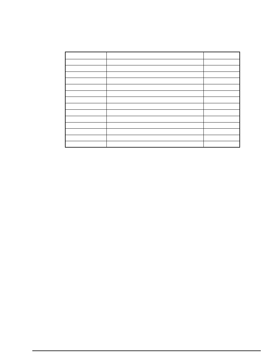
Programmer's Tutorial / CD-ROM Library
12-25
Error Codes
Table 12-1 Error Codes
Constant name
Meaning
Constant value
CDERR_OK
Normal end
(0)
CDERR_RDERR
Read error
(-1)
CDERR_NODISC
Disc not loaded
(-2)
CDERR_CDROM
Disc not a CD-ROM
(-3)
CDERR_IPARA
Illegal initialization parameter
(-4)
CDERR_DIR
Change attempted to structure that was not a directory
(-6)
CDERR_NEXIST
File not found
(-9)
CDERR_NUM
Negative byte count
(-14)
CDERR_PUINUSE
Pickup in operation
(-20)
CDERR_ALIGN
Work area not a multiple of four bytes
(-21)
CDERR_TMOUT
Timeout
(-22)
CDERR_OPEN
Tray open
(-23)
CDERR_FATAL
CD drive status: "FATAL"
(-25)
CDERR_BUSY
Status in transition
(-50)
|

Programmer's Tutorial
13
Backup Library
The Sega Saturn system has a 32K internal buffer memory. This chapter
explains the backup library provided in order to use this internal buffer
memory.
The backup library itself is compressed and stored in the Sega Saturn
boot ROM.
This backup library can be used to transfer data between buffer memory
and external cartridges.
|

13-2
Programmer's Tutorial / Backup Library
Features of the Backup Library
Devices
Supported devices
The backup library can access devices (currently limited to the internal backup memory and
external cartridges) with a non-hierarchical file format. (Table 13-1.) Furthermore, these
devices are partitioned as shown in Fig. 13-1.
Device connection information (Config)
The connection (Config) information of each device can be gotten during the initialization
processing of the backup library.
Information on each device (Status: connected/not connected, formatted/
unformatted, etc.)
Status information can be gotten by using a backup library function. In addition, it is possible
to specify the size of a file that you want to write and determine whether or not it is possible to
write a file of that size.
Table 13-1 Device List
Device Number
Device type
0
Internal memory cartridge
1
Memory cartridge or parallel interface
Fig 13-1 Device Configuration
Backup library
·
Config
·
Status
·
Dir
·
Dir
Device
Partition
File
Partition
File
Device
|

Programmer's Tutorial / Backup Library
13-3
Files
Information on each file (Dir: name, creation date, etc.) can be gotten by using a backup library
function.
When a file is created, the file information is set as desired by the user; the backup library itself
does not create the file information.
Library expansion
The backup library is stored in compressed form within the Sega Saturn Boot ROM. When the
user uses the backup library, it allocates a program expansion area and work area and then
performs initialization processing. All of the functions can be used as desired thereafter.
Note: If backup library processing is interrupted while data is being written, the data is
destroyed. Therefore, whenever you are performing backup library initialization,
formatting, writing, or deletion processing, use the system library function
"slResetDisable()" (peripheral function) to disable the reset button.
|

13-4
Programmer's Tutorial / Backup Library
Basic Flow of Processing
The backup library functions are explained below in accordance with the basic flow of processing.
1) Initialization [BUP_Init()]
This function reads the backup library from the boot ROM and expands it in the specified
address space. The device information at that time is returned.
2) Select partition (BUP_SelPart()]
This function specifies the device partition to be used. The default partition is No. 0 (inter-
nal memory cartridge).
3) Get status [BUP_Stat()]
This function gets the status of the device to be written/read. When writing, specify the
number of bytes of data to be written; the return value will indicate whether that much data
can be written to the device or not.
4) Format (BUP_Format()]
After getting the status, if it is discovered that the device to be used is unformatted, it is
necessary to first format the device. Formatting is limited to the specified partition in the
specified device.
5) Get directory information [BUP_Dir()]
This function gets the directory information for the specified file name (or for all files). If
the directory information for all files is desired, specify "NULL" for the file name.
6) Write data [BUP_Write()]
This function writes a file to the specified device. The necessary file information must be
created by the user.
7) Verify data [BUP_Verify()]
This function verifies a file written to the specified device.
8) Read data [BUP_Read()]
This function reads a file written on a specified device.
9) Delete data [BUP_Delete()]
This function deletes a file from the specified device.
10) Expand date data [BUP_GetDate()]
This function expands the date data stored in the compressed file information.
11) Compress date data (BUP_GetDate()]
This function compresses and stores the date data in the file information.
|

Programmer's Tutorial / Backup Library
13-5
Sample Program
The following flow chart shows the flow of operations in the sample program that uses the
backup library.
Flow Chart 13-1 Backup Library Sample Program
START
END
Initialize
Get status
Format
Create directory
information
Get file
information
Get status
Write file
Get file information
for all files
Get file information
for all files
Verify
Read file
Delete file
Unformatted?
Can data
be written?
No
No
Yes
Yes
|

13-6
Programmer's Tutorial / Backup Library
List 13-1 is the program listing for the sample program.
List 13-1 Sample Program
#include
"sgl.h"
#include
"sega_per.h"
#define
BUP_STAT_ADDR
0x6070000
#include
"sega_bup.h"
#define FILE_NAME"FILE_NAME01"
#define BACKUP_DEVICE(Uint32)0
#define TEST_DATA"It's a pen"
#define TEST_SIZE 10
#define DIR_SIZE 8
/****************************************
*****************************************/
/**************************************
***************************************/
void
BackUplnit(BupConfig cntb|3|)
{
Uint32
BackUpRamWork|2048|;
slResetDisable();
BUP_Init((Uint32*)BUP_STAT_ADDR.BackUpRamWork.cntb):
slResetEnable();
}
/*************************
*
**************************/
Sint32
BackUpWrite(Uint32 device, BupDir*dir, Uint8 *data, Uint8 sw)
{
Sint32
ret;
SmpcDateTime
*time;
BupDate date;
if(!dir->date){
time=&(Smpc_Status->rtc);
date.year=(Uint8)(slDec2Hex(time->year)-1980);
date.month=(Uint8)(time->month&0x0f);
date.week=(Uint8)(time->month>>4);
date.day=(Uint8)(time->date);
date.time=(Uint8)(time->hour);
date.min=(Uint8)(time->minute);
dir->date=BUP_SetDate(&date);
}
slResetDisable();
ret=BUP_Write(device,dir,data,sw);
slResetEnable();
return(ret);
}
/**************************/
/*
/**************************/
Sint32
BackUpDelete(Uint32 device,Uint8 *filename)
{
Sint32 ret;
slResetDisable();
ret=BUP_Delete(device,filename);
slResetEnable();
return(ret);
}
/* specification of address where library is to be expanded */
/* use internal memory */
/* reset button disabled */
/* reset button enabled */
/* if date data is "0", input current date */
/* get date data */
/* reset button disabled */
/* reset button enabled */
/* reset button disabled */
/* reset button enabled */
Backup RAM sample program
* Library initialization processing *
Write processing *
Deletion processing */
|

Programmer's Tutorial / Backup Library
13-7
Listing 13-1 Sample Program (continued)
/**************************/
/*
/**************************/
Sint32
BackUpFormat(Uint32 device)
{
Sint32 ret;
slResetDisable();
ret = BUP_Delete(device);
slResetEnable();
return(ret);
}
void
main()
{
BupConfig
conf[3];
BupStat
sttb;
BupDir
dir,dirs[DIR_SIZE];
BupDate
datetb,date;
Uint8 *time;
Sint32 status;
Uint8 buf[256];
int
i;
slInitSystem(TV_352x224,(TEXTURE*)NULL.1);
slGetStatus();
for(i=0;i<100;i++)
{
slSynch();
}
BackUpInit(conf);
if(( status=BUP_Stat(BACKUP_DEVICE.10.&sttb))==BUP_UNFORMAT )
{
status=BackUpFormat(BACKUP_DEVICE);
BUP_Stat(BACKUP_DEVICE.TEST_SIZE,&sttb);
}
if( sttb.freeblock>0)
{
stmcpy(dir.filename. FILE_NAME,11);
stmcpy(dir.comment. "Test.desu".10);
dir.language=BUP_ENGLISH;
dir.datasize=TEST_SIZE;
dir.date = 0;
status=BackUpWrite(BACKUP_DEVICE.&dir.(Uint8*)TEST_DATA.OFF);
status=BUP_Verify(BACKUP_DEVICE.(Uint8*)FILE_NAME.(Uint8*)TEST_DATA):
}
status=BUP_Dir(BACKUP_DEVICE.(Uint8*)FILE_NAME DIR_SIZE.dirs):
status=BUP_Dir(BACKUP_DEVICE.(Uint8*)"".DIR_SIZE.dirs):
status=BUP_Read(BACKUP_DEVICE.(Uint8*)FILE_NAME.buf):
status=BackUpDelete(BACKUP_DEVICE.(Uint8*)FILE_NAME):
status=BUP_Dir(BACKUP_DEVICE.(Uint8*)"",DIR_SIZE.dirs):
}
Format processing */
/* reset button disabled */
/* reset button enabled */
/* get time */
/* initialization processing */
/* get status */
/* format */
/* write */
/* verify */
/* directory information */
/* all directory information */
/* read */
/* delete */
/* all directory information */
|

13-8
Programmer's Tutorial / Backup Library
Supplement. Backup Library functions
Table 13-2 lists the functions used in the backup library.
For details on the functions, refer to the PROGRAMMER'S GUIDE, vol. 1.
Table 13-2 Backup Library Functions
Number
Function Name
Function
1
BUP_Init
Initializes backup library
2
BUP_SelPart
Selects partition
3
BUP_Format
Executes formatting operation
4
BUP_Stat
Gets status
5
BUP_Write
Writes data
6
BUP_Read
Reads data
7
BUP_Delete
Deletes data
8
BUP_Dir
Gets directory information
9
BUP_Verify
Verifies data
10
BUP_GetDate
Expands date data
11
BUP_SetDate
Compresses date data
|

Sound Library
This chapter describes the procedures and cautions relevant to
outputting sound on the Sega Saturn system using the sound
control library.
Programmer's Tutorial
14
|

14-2
Programmer's Tutorial / Sound Library
Sound Control Overview
The Sega Saturn system is equipped with an MC68000 as a sound control CPU that is capable
of operating independently of the master CPU.
The master CPU and the sound CPU exchange functions through a portion of RAM called the
"command buffer." Because the functions are issued by the sound control library, sound is
controlled without the user being aware of the interactions between the CPUs.
The sound sources that can be used with the Sega Saturn system are PCM and CDs; the sound
driver controls PCM sound sources.
Fig 14-1 Sound Driver System Configuration
PCM
sound
source
Sound
library
Main RAM
Master
CPU
Slave
CPU
Sound
driver
Sound
data
Command
buffer
Shared RAM
MC68000
Sound CPU
|

Programmer's Tutorial / Sound Library
14-3
Sound Driver Setup
The following procedure is required in order to use the sound driver to control sound in the
Sega Saturn system.
Fig 14-2 Sound Control Procedure
Driver setup and
MC68000 startup
Sound data setup
BGM (background music)
playback/sound effects,
PCM sound source control
Sound driver setup and MC68000 startup
In order to use sound, it is first essential to start up the MC68000 that is used to control sound.
The driver program that runs on the MC68000 is also needed. This program can be set up by
executing the library function "slInitSound()".
[void slInitSound (void *drv, Uint32 drvsz, void *map, Uint32 mapsz);]
This function sets up the sound driver and initializes the sound CPU (MC68000). "drv" is
the sound driver program that runs on the MC68000, and is loaded into the area starting from
address 0 in the MC68000. "drvsz" is the size of the driver program.
Normally, this function is specified as follows:
slInitSound (drv, sizeof(drv), maptbl, sizeof(maptbl));
The "slInitSound" function executes the following sequence of operations:
1) Reset MC68000.
2) Clear with zeroes the memory area up to address 0xB000 in the MC68000.
3) Transfer the driver program (size starting from address 0).
4) Transfer map data (size starting from address 0xA000).
5) Register memory area for PCM playback.
6) Start up MC68000.
7) Register map data.
|

14-4
Programmer's Tutorial / Sound Library
Sound data setup
Because executing only the "slInitSound" function described above does not set up the playback
data, it is necessary to do so now. The playback data is stored starting from address 0xB000 in
the MC68000 memory area (0x25A0B000 in the program). (These addresses may vary, de-
pending on the map data; consult with the sound designer.) Use the following function to
transfer the data:
Fig 14-3 Sound Data Setup Example
slDMACopy(sounnad,(voied*)0x25a0b000,sizeof(sounddat));
slDMAWait();
Preparations for playback are now complete.
Background music playback
Music (and sound effects) are handled in units called "sequences." A sequence is the playback
of a series of sound combinations from start to finish (and can either be an entire song or a
single sound effect). With the Sega Saturn sound driver, up to eight sequences can be played
back simultaneously. In the SGL, of these eight sequences, No. 0 is allocated for background
music. To play background music, execute the function "slBGMOn()".
[Bool slBGMOn (Uint16 Song, Uint8 Prio, Uint8 Volume, Uint8 Rate);]
This function starts background music playback.
Song:
Song (sound effect) number
Prio:
Priority for using the sound source
Volume:
Volume
Rate:
Time until the volume is reached
"Prio" is the priority for using the sound source. Because the 32-channel sound source is
shared by multiple sequences for sound output, if the total number of channels being sued
exceeds 32, sounds with the lowest priority numbers are not allocated channels.
The volume ("Volume") can be set from 0 to 127, with a higher value representing a louder
volume. The rate ("Rate") is the time taken to reach that volume, and can be specified with a
value from 0 to 255. Specifying "0" means that the volume is reached immediately, while a
value from 1 to 255 causes the volume to fade in from the 0 level to the specified level.
The following functions can be used to change the tempo and volume of the background music
and to stop, pause, and resume playback.
slBGMTempo (Sint16, Tempo)
/* change tempo */
slBGMFade (Uint8 Volume, Uint8 Rate);
/* change volume */
slBGMOff();
/* stop playback */
slBGMPause();
/* pause playback */
slBGMCont();
/* resume playback */
slBGMStat();
/* check to determine if playback is in progress */
|

Programmer's Tutorial / Sound Library
14-5
Sound effect output
Just as with background music, sound effects are also managed as sequences. To output a
sound effect, execute the function "slSequenceOn()".
[Uint8 slSequenceOn (Uint 16 Song, Uint8 Prio, Uint8 Volume, Uint8 Pan);]
Song:
Song (sound effect) number
Prio:
Priority for using the sound source
Volume:
Volume
Pan:
Left-right balance of volume
The parameters resemble those for the BGM function, except for the parameter "Pan". This
parameter represents the left-right balance of the volume, and can be used to give a sound
directionality. A value ranging from -128 to +127 can be specified for "Pan", with -128
representing the left, 0 representing the middle, and +127 representing the right.
Substitution values for the parameter "Pan":
Left: -128 << 0 >> +127: Right
By using the "Volume" and "Pan" settings, sound can be used to create illusions of distance and
directionality in games.
The function "slSequenceOn()" returns the sound control number that the specified sound effect
is being output under. This sound control number can be used to alter the corresponding sound
effect with the following functions:
slSequenceTempo (Uint8 Seqnm, Sint16 Tempo);
/* change tempo */
slSequenceFade (Uint8 Seqnm, Uint16 Volume, Uint8 Rate);
/* change volume */
slSequencePan (Uint8 Seqnm, Uint8 Pan);
/* change directionality */
slSequenceOff (Uint8 Seqnm);
/* stop sequence */
slSequencePause (Uint8 Seqnm);
/* pause sequence */
slSequenceCont (Uint8 Seqnm);
/* resume paused sequence */
slSequenceStat (Uint8 Seqnm);
/* check to determine if sequence is being played back */
Outputting sound effects using the PCM sound source
The PCM sound source can be used when outputting sound effects created by audio sampling
(voices, explosions, etc.). Unlike the sequences described above, sound effect playback via
PCM stream can be output on a maximum of four channels. When using the PCM stream,
execute the function "slPCMOn()".
[Sint8 slPCMOn (PCM *pdat, void *data, Uint32 size);]
This function starts playback using the PCM sound source.
pdat: PCM-type structure data for PCM stream playback mode, etc.
data: PCM stream sound source data
size: PCM stream data size
|

14-6
Programmer's Tutorial / Sound Library
The organization of the PCM-type structure data is shown below; this data is used to specify the
PCM stream playback parameters.
Fig 14-4 PCM-type Structure Data
typedef struct{
Uint8 mode;
Uint8 channel;
Uint8 level;
Sint8 pan;
Uint16pitch;
Uint8 eflevelR;
Uint8 efselectR;
Unit8 eflevelL;
Uint8 efselectL;
}PCM;
/* Mode */
/* PCM Channel Number */
/* 0
-
127 */
/* -128
-
+127 */
/* Effect level for Right(mono) 0- 7 */
/* Effect select for Right(mono) 0- 15*/
/* Effect level for Left 0
-
7 */
/* Effect select for Left 0
-
15 */
Specify "_Stereo" or "_Mono" and "_PCM16Bit" or "_PCM8Bit".
PCM playback channel (set by this function)
Volume
Left-right balance of volume
Playback rate (changes pitch)
Extent of applied effect (right channel)
Effect number (right channel)
Extent of applied effect (left channel)
Effect number (left channel)
mode:
channel:
level:
pan:
pitch:
eflevelR:
efselectR:
eflevelL:
efselectL:
Because PCM streams are played back as the master CPU sets the data that is used by the sound
SCSP LSI, unlike the sequences described earlier, the load on the master CPU increases.
Consult with the sound designer in order to determine whether sound is to be output using the
sequences described earlier or by using PCM streams. The function "slPCMOn()" returns the
control number that the specified PCM stream is being output under.
Other functions that are used for PCM stream sound effect playback are listed below.
slPCMOff (PCM *pdat);
/* stop playback */
slPCMParmChange (PCM *pdat);
/* change parameter */
slPCMStat (PCM *pdat);
/* check to determine if playback is in progress on specified PCM channel */
Functions that affect sound output as a whole
The functions described up to this point affect individual sound outputs; the following functions
affect sound output as a whole.
slSndVolume (Uint8 Volume);
/* overall volume */
slSoundAllOff();
/* stop all sound sequences */
slDSPOff();
/* stop effect DSP */
slSndMixChange (Uint8 Tbank, Uint8 Mixno);
/* switch mixer */
slSndMixParmChange (Uint8 Effect, Uint8 Level, Uint8 Pan);
/* change mixer parameters */
|

Programmer's Tutorial / Sound Library
14-7
Memory Map
The figure below shows a general memory map for the sound CPU. If PCM streams are not
used, the PCM playback buffer can be used for sequence data since it is not needed for PCM
streams.
Fig 14-5 Sound CPU Memory Map
Exception vectors, etc.
Command buffer
Pitch, sequence
Current map data
Map data
Sound driver
PCM playback buffer
25A00000:
25A00500
25A00700
25A00800
25A0A000
25A0B000
25A78000
25A7FFFF
|

14-8
Programmer's Tutorial / Sound Library
Sample Program
Sample program for playback test of background music and sound effects
The following sample program is designed for a playback test of background music and sound
effects. The organization of the data file used for this sample program is shown below.
Fig 14-6 Sample Program Data File
Bank
Song
Contents
0
0
1
1
0
Song (no loop)
Song (with loop)
Sound effect (C3)
1
Sound effect (D3)
2
Sound effect (E3)
3
Sound effect (F3)
4
Sound effect (G3)
5
Sound effect (A3)
6
Sound effect (B3)
7
Sound effect (C4)
2
0
Cheer
3
0
Long violin sound
1
Short violin sound (loop)
The songs specified by "bank" and "song" are played back as background music when the X
button is pressed, and as a sound effect when the A button is pressed. The "bank" and "song"
specifications are made using the Start key and the direction key.
The Y and B buttons are used to pause and resume each of the background music and sound
effects, and the Z and C buttons are used to fade in and out.
The sound effect sequence number specification is made by using the using the direction key in
the left/right direction, and the overall volume is set by using the direction key in the up/down
direction.
List 14-1 sampsnd1: Background Music and Sound Effect Playback Test
- sampsnd1 -
/*
*/
/* Sound control sample
*/
/*
*/
#include "sl_def.h"
#include "sddrvs.dat"
/*----------------------------------------------*/
#define SoundSeqBuf
0x25a06000
extern char sound_map[];
extern char sound_dat[];
extern Uint32 mapsize;
extern Uint32 datasize;
extern PDATA PD_Cube;
/*----------------------------------------------*/
/* include files containing various settings */
/* sound driver file */
/* sequence buffer address */
|

Programmer's Tutorial / Sound Library
14-9
List 14-1 sampsnd1: Background Music and Sound Effect Playback Test
(continued)
#define _Play
0x01
#define _Pause
0x02
#define _Fade
0x04
typedef struct{
struct{
Sint8
stat;
Sint16
tmp;
sint8
pan;
}seq|8|;
Uint8 banknum ;
Uint8 songnum ;
Uint8 sequence ;
}SOUND_MAN;
/*----------------------------------------*/
void init_sound(){
slInitSound(sddrvstsk, sizeof(sddrvstsk),(Uint8*)sound_map, mapsize);
slDMACopy(sound_dat,(void*)(SoundSeqBuf),datsize);
}
void disp_vol(Uint16 vol){
slSndVolume(vol<<3);
slPrint("Volume:",slLocate(2.6)):
slPrintHex(vol, slLocate(11.6));
}
sound_test(EVENT*evptr){
SOUND_MAN
*smptr;
PerDigital
*pptr;
Sint16
padd;
Sint16
padp;
int i :
const Uint8 bank = 3 ;
const Uint8 song{}={1,7,0,1};
smptr=(SOUND_MAN*)evptr->user;
pptr=Smpc_Peripheral;
padd="pptr->data;
padp="pptr->push;
/* status mode define */
/* driver/map transfer */
/* transfer sound data to sequence buffer */
/* set/display volume */
/* number of banks included in "sampdat.c" */
/* number of songs in each bank */
|

14-10
Programmer's Tutorial / Sound Library
List 14-1 sampsnd1: Background Music and Sound Effect Playback Test
(continued)
for (i = 7: i>=();i--){
if(smptr->seq|i|stat &&!(slSequenceStat(i))){
smptr->seq|i|stat=();
}
switch(smptr->seq{i}.stat)(
case0:slPrint(" ", slLocate(33.3+i));break ;
case1:slPrint("Play ", slLocate(33.3+i));break ;
case3:slPrint("Pause ", slLocate(33.3+i));break ;
case5:slPrint("Fade Out", slLocate(33.3+i));break;
case7:slPrint("Pause ", slLocate(33.3+i));break;
{
}
if(padd & PER_DGT_ST){
if(padd & PER_DGT_KU){
if(++smptr->banknum>bank)smptr->banknum=0;
if(smptr->songnum>song|smptr->banknum|)smptr->songnum=song|sinptr->banknum|:
}else if(padp & PER_DGT_KD){
if(--smptr->banknum > bank) smptr->banknum = bank;
if(smptr->songnum>song|smptr->banknum|)smptr->songnum=song|smptr->banknum|;
}
if(padp & PER_DGT_KR){
if(++smptr->songnum > song|smptr->banknum|)smptr->songnum = ();
}else if(padp & PER_DGT_KL){
if(--smptr->songnum>song|smptr->banknum|)smptr->songnum=song|smptr->banknum|;
}
}else{
if(padp & PER_DGT_KU){
if(smptr->vol <15){
disp_vol(++smptr->vol);
}
} else if(padp & PER_DGT_KD){
if(smptr->vol >()){
disp_vol(++smptr->vol);
}
{
if(pade & PER_DGT_KR){
if(++smptr->sequence> 7)smptr->sequence=1;
} else if(pade & PER_DGT_KL){
if(--smptr->sequence< 1)smptr->sequence=7;
}
}
slPrintHex(slHex2Dec(smptr->banknum), slLocate(7.10)):
slPrint("Bank :",slLocate(2.10));
slPrintHex(slHex2Dec(smptr->songnum), slLocate(7.11)):
/* check for end of sequence playback */
/* if playback is complete, clear status flag to "0" */
/* display message according to status flag */
/* direction key input while Start button is pressed */
/* Bank/song/sequence display */
/* direction key input while Start button is not pressed */
|

Programmer's Tutorial / Sound Library
14-11
List 14-1 sampsnd1: Background Music and Sound Effect Playback Test
(continued)
slPrint("Song :", slLocate(2.11)):
slPrintHex(slHex2Dec(smptr->sequence), slLocate(7.12)):
slPrint("Sequence:", slLocate(2.12)):
if(padp & PER_DGT_TX){
if(smptr->seq|()|.stat=&_Play){
slBGMOff():
smptr->seq|0|.stat=0;
}else {
slBGMOn(smptr->banknum<<8)+smptr->songnum,(0,127.0)
smptr->seq|0|.stat:=_Play ;
}
}
if(pade & PER_DGT_TA){
if(smptr->seq|smptr->sequence|.stat *_Play){
slSequenceOff(smptr->sequence);
smptr->seq|smptr->sequence|.stat=0;
}else {
smptr->seq|slSequenceOn(smptr->banknum<<8)+smptr->songnum.0.1270)|.stat:=_Play :
}
}
if(smptr->seq|0|.stat &_Play){
if(pade & PER_DGT_TY){
if(smptr->seq|0}.stat &_Pause){
slBGMCont();
smptr->seq|0|.stat & ="(_Pause);
} else {
slBGMPause();
smptr->seq|0|.stat:=_Pause;
}
}
if(!(smptr->seq|0|.stat &_Pause)){
if(pade & PER_DGT_TZ){
if(smptr->seq|0|.stat &_Fade){
smptr->seq|0|.stat &="(_Fade);
slBGMFade(127.25);
} else {
smptr->seq|0|.stat :=Fade ;
slBGFade(1.25);
}
}
}
}
if(smptr->seq|smptr->sequence|.stat &_Play){
if(padp & PER_DGT_TB){
if(smptr->seq|smptr->sequence|.stat &_Pause){
if(smptr->seq|0|.stat &_Pause){
slSequenceCont(smptr->sequence);\
smptr->seq|smptr->sequence|.stat &="(_Pause);
} else {
slSequencePause(smptr->sequence);
smptr->seq|smptr->sequence|.stat:=_Pause;
}
}
if(!(smptr->seq|smptr->sequence|.stat &_Pause)){
if(padp & PER_DGT_TC){
if(smptr->seq|smptr->sequence|.stat &_Fade){
smptr->seq|smptr->sequence|.stat &="(_Fade);
slSequenceFade(smptr->sequence . 127.25);/*Fade ln*/
} else {
smptr->seq|smptr->sequence|.stat:=Fade;
slSequenceFade(smptr->sequence . 1.25);
}
}
}
}
}
/* X button input */
/* background music on/off */
/* A button input */
/* sound effect on/off */
/* background music is playing... */
/* Y button input */
/* pause on/off */
/* if not paused... */
/* Z button input */
/* fade in/out */
/* Fade In */
/* Fade Out */
/* if sound effect of specified sequence is not being played... */
/* B button input */
/* pause on/off */
/* if pause is not on... */
/* C button input */
/* fade in/out */
/* Fade Out */
|

14-12
Programmer's Tutorial / Sound Library
List 14-1 sampsnd1: Background Music and Sound Effect Playback Test
(continued)
void init_sound_test(EVENT*evptr){
SOUND_MAN *smptr;
inti;
evptr->exad=(void *)sound_test;
smptr=(SOUND_MAN *)evptr->user;
smptr->vol=15;
smptr->sequence=1;
smptr->danknum=0;
smptr->songnum=0;
for(i=7;i>=0;i--){
smptr->seq|i|.stat=0;
slPringHex(i.slLocate(24.3+i));
}
disp_vol(smptr->vol);
}
/*---------------------------------------------*/
typedef struct{
ANGLEangy;
}CUBE_MAN;
void disp_cube(EVENT*evptr){
CUBE_MAN
*cbptr;
cbptr=(CUBE_MAN*)evptr->user;
slPushUnitMatrix();
{
slTranslate(toFIXED(0),toFIXED(0),toFIXED(500));
slRotY(cbptr->angy);
cbptr->angy+=0x0|00;
slPutPolygon(&PD_Cube);
}
slPopMatrix();
}
/*---------------------------------------------*/
sample(){
init_sound();
slInitEvent();
slSetEvent((void*)init_sound_test);
slSetEvent((void*)disp_cube);
slScrAutoDisp(NBG0ON);
slPrint("Sound test",slLocate(10.2));
while(-1){
slExecuteEvent();
slSynch();
}
}
/*---------------------------------------------*/
void main(){
slInitSystem(TV_352x224,NULL,1);
sample();
}
/*---------------------------------------------*/
/* data initialization */
/* cube display */
/* title display */
|

Programmer's Tutorial / Sound Library
14-13
Flow Chart 14-1 sampsnd1: Background Music and Sound Effect Playback Test
Initialize system
Background
music on/off
Sound effect
on/off
Pause on/off
Fade in/out
Pause on/off
Fade in/out
Transfer sound data
to sequence buffer
Set sound driver
Initialize data
Display cube
Register event
Check sequence
status
Is direction
key being pressed
(up/down)?
Is Start key
being pressed?
Is X button
being pressed?
Is background
music playing?
Not paused?
Not paused?
Is sound effect
indicated by variable
"sequence" being
played back?
Is A button
being pressed?
Is Y button
being pressed?
Is Z button
being pressed?
Is C button
being pressed?
Is B button
being pressed?
Is direction
key being pressed
(up/down)?
Is direction
key being pressed
(left/right)?
Is direction
key being pressed
(left/right)?
No
No
No
No
No
No
No
No
No
No
No
No
No
No
No
Yes
Yes
Yes
Yes
Yes
Yes
Yes
Yes
Yes
Yes
Yes
Yes
Yes
Yes
Yes
Change volume
Change sequence
number
Change bank
number
Change song
number
Display bank, song,
and sequence number
|

14-14
Programmer's Tutorial / Sound Library
Sample program for playback test of PCM sound source
The following sample program is designed for a playback test of the PCM sound source.
There are three types of PCM sound source sample data: 16-bit stereo, 8-bit stereo, and 16-bit
monaural. Each is played back by pressing the X button, Y button, and Z button, respectively.
List 14-2 sampsnd2: PCM Sound Source Playback Test
-sampsnd2-
/*
*/
/* Sound control sample
*/
/*
*/
#include
"sl_def.h"
#include
"sddrvs.dat"
/*---------------------------------*/
extern char s_16{};
extern Uint32 s_16_size;
extern PCM s_16_dat;
extern char s_8{};
extern Uint32 s_8_size;
extern PCM s_8_dat;
extern char m_16{};
extern Uint32 m_16_size;
extern PCM m_16_dat;
extern PDATA PD_Cube;
/*--------------------------------*/
void init_sound(){
char sound_map{}=(0xff,0xff};
slInitSound(sddrvstsk, sizeof(sddrvstsk),(Uint8*)sound_map, sizeof(sound_map));
}
sound_test(EVENT*evptr){
PerDigital*pptr;
Sint16
pad;
pptr=Smpc_Peripheral;
pad="pptr->push; /* Push data*/
if(pad & PER_DGT_TX){
slPCMOn(&s_16_dat,s_16,s_16_size);
}
/* include files containing various settings */
/* sound driver file */
/* dummy map setting */
/* driver map transfer */
/* X button input */
/* Stereo_16Bit playback */
|

Programmer's Tutorial / Sound Library
14-15
List 14-2 sampsnd2: PCM Sound Source Playback Test (continued)
if(pad & PER_DGT_TY){
slPCMOn(&s_8_dat,s_8,s_8_size);
}
if(pad & PER_DGT_TZ){
slPCMOn(&m_16_dat,m_16,m_16_size);
}
}
/*-----------------------------------*/
typedef struct{
ANGLEangy;
}CUBE_MAN;
void disp_cube(EVENT*evptr){
CUBE_MAN
*cbptr;
cbptr=(CUBE_MAN*)evptr->user;
slPushUnitMatrix();
{
slTranslate(toFIXED(0),toFIXED(0),toFIXED(500));
slRotY(cbptr->angy);
cbptr->angy+=0x0100;
slPutPolygon(&PD_Cube);
}
slPopMatrix();
}
/*--------------------------------*/
sample(){
init_sound();
slInitEvent();
slSetEvent((void*)sound_test);
slSetEvent((void*)disp_cube);
slScrAutoDisp(NBG0ON);
slPrint("Sound PCM test",slLocate(10.2));
while(-1){
slExcuteEvent();
slSynch();
}
}
/*-------------------------------*/
void main(){
slInitSystem(TV_352x224,NULL,1);
sample();
}
/*--------------------------------*/
/* Y button input */
/* Stereo_8Bit playback */
/* Z button input */
/* Mono_16Bit playback */
/* cube display */
/* title display */
|

14-16
Programmer's Tutorial / Sound Library
Flow Chart 14-2 sampsnd2: PCM Sound Source Playback Test
Initialize system
Set up
sound driver
Register event
Stereo_16Bit
playback
Stereo_8Bit
playback
Mono_16Bit
playback
Display cube
Is X button
being pressed?
Is Y button
being pressed?
Is Z button
being pressed?
Yes
No
No
No
Yes
Yes
|

Programmer's Tutorial / Sound Library
14-17
Supplement. Sound Library Functions Appearing in This Chapter
The following functions were covered in this chapter.
Table 14-1 Sound Driver Functions Appearing in This Chapter
Function type
Name
Parameters
Function
void
slInitSound
void *drv, Uint32 drvsz,
Setup sound driver and initialize sound
void *map, Uint32 mapsz
CPU
Bool
slBGMOn
Uint16 Song, Uint8 Prio,
Start background music playback
Uint8 Volume, Uint8 Rate
Bool
slBGMTempo
Sint16 Tempo
Change background music playback
speed
Bool
slBGMFade
Uint8 Volume, Uint8 Rate
Change background music playback
volume
Bool
slBGMOff
void
Stop background music playback
Bool
slBGMPause
void
Pause background music playback
Bool
slBGMCont
void
Resume playback of paused background
music
Bool
slBGMStat
void
Check to determine if background music
is being played back
Unit8
slSequenceOn
Uint16 Song, Uint8 Prio,
Start generating specified sound effect
Uint8 Volume, Uint8 Pan
Bool
slSequenceTempo
Uint8 Seqnm, Sint16 Tempo
Change speed of specified sound effect
Bool
slSequenceFade
Uint8 seqnm, Unit8 Volume,
Change volume of specified sound effect
Uint8 Rate
Bool
slSequencePan
Uint8 Seqnm, Uint Pan
Change directionality of specified sound
effect
Bool
slSequenceOff
Uint8 Seqnm
Stop specified sound effect
Bool
slSequencePause
Uint8 Seqnm
Pause specified sound effect
Bool
slSequenceCont
Uint8 Seqnm
Resume paused sound effect
Bool
slSequenceStat
Uint8 Seqnm
Check to determine if specified sound
effect is being played back
Sint8
slPCMOn
PCM *pdat, void *data,
Start PCM sound source playback
Uint32 size
Bool
slPCMOff
PCM *pdat
Stop PCM sound source playback
Bool
slPCMParmChange
PCM *pdat
Change PCM playback parameters
Bool
slPCMStat
PCM *pdat
Check playback on specified PCM
channel
Bool
slSndVolume
Uint8 Volume
Set overall volume
Bool
slSoundAllOff
void
Stop playback of all sound sequences
Bool
slDSPOff
void
Stop DSP playback
Bool
slSndMixChange
Uint8 Tbank, Uint8 Mixno
Switch mixer corresponding to tone bank
Bool
slSndMixParmChange
Uint Effect, Uint8 Level, Uint8
Pan Change mixer parameters
|

Designer's Tutorial
The Sega Saturn Designer's Tutorial is designed to
provide the knowledge required of designers in the
development of 3D software for the Sega Saturn
system.
This manual assumes that the design work is per-
formed using SOFTIMAGE, and uses actual ex-
amples based on this software to explain the neces-
sary procedures for creating 3D models. Because
this manual also explains basic concepts of 3D mod-
els, it can be used even by designers with no 3D
design work experience.
|

1
Table of Contents
Introduction ................................................................. 1-1
What is a 3D Model? ............................................................................. 1-2
Polygons ............................................................................................ 1-2
Texture mapping ................................................................................ 1-2
Basic Operation of SOFTIMAGE .......................................................... 1-3
Before starting up SOFTIMAGE (creating the directory) ................... 1-3
SOFTIMAGE startup .......................................................................... 1-3
Database creation.............................................................................. 1-4
The screen ......................................................................................... 1-5
Displaying 3D models ........................................................................ 1-7
Saving data ........................................................................................ 1-8
Loading data ...................................................................................... 1-8
Modeling Training: Beginning Level "TV Monitor" ... 2-1
Setting the mode................................................................................ 2-2
Getting a cube ................................................................................... 2-2
Changing the viewpoint ..................................................................... 2-3
Displaying the Vertices ...................................................................... 2-4
Adding middle vertices ....................................................................... 2-4
Adding edges ..................................................................................... 2-5
Removing vertices ............................................................................. 2-5
Removing edges ................................................................................ 2-6
Tag selection ..................................................................................... 2-7
Switching the operation mode ........................................................... 2-8
Scaling (enlargement/reduction) ........................................................ 2-8
Duplicating polygons .......................................................................... 2-9
Polygon movement (Trans) ............................................................... 2-9
Shaded display ................................................................................ 2-10
Object scaling .................................................................................. 2-11
Inputting the scale ratio value .......................................................... 2-11
Checking the coordinates of vertices ............................................... 2-14
Dividing polygons............................................................................. 2-18
Modeling Training: Advanced Level "Automobile" .. 3-1
Creating the Fundamental Shape of the Car ........................................ 3-2
Getting a cube ................................................................................... 3-2
Creating the base .............................................................................. 3-3
Creating the roof ................................................................................ 3-4
Adjusting the roof ............................................................................... 3-6
Adjusting the body of the car ............................................................. 3-8
Creating the Wheel Wells.................................................................... 3-11
|

2
Creating indentations ....................................................................... 3-11
Deleting unnecessary surfaces ........................................................ 3-13
Creating the Wheels ............................................................................ 3-14
Getting a cylinder ............................................................................. 3-14
Using the Schematic screen ............................................................ 3-14
Shaping the cylinder ........................................................................ 3-16
Preparing the surface ...................................................................... 3-18
Adjusting the wheel.......................................................................... 3-22
Wheel placement ............................................................................. 3-25
Finishing Touches for the Model ......................................................... 3-28
Creating polygon surfaces ............................................................... 3-28
Dividing polygons............................................................................. 3-30
Deleting polygons ............................................................................ 3-31
Adding details to the body ............................................................... 3-33
Positioning the wheels ..................................................................... 3-40
Completing the Car ............................................................................. 3-41
Combining the car and wheels into a single object
(parent-child structure) ..................................................................... 3-41
Final check ...................................................................................... 3-42
Coloring the Model ...................................................... 4-1
Preparation before coloring ............................................................... 4-2
Material assignment........................................................................... 4-2
Apply color to entire object ................................................................ 4-3
Applying color to the monitor screen frame ....................................... 4-5
Coloring the monitor screen............................................................... 4-8
Supplement: Color Setting Chart Used by the Saturn System ............. 4-9
Useful Techniques....................................................... 5-1
Merge and Clean Up (Using Left-Right Symmetry in Modeling) ........... 5-2
Magnet Function (Point-to-Point Attraction Function) ........................... 5-8
Dividing a Polygon When an Edge Cannot be Drawn ......................... 5-16
Preparations (creating a polygon).................................................... 5-16
Solution 1: Create a triangle at the edge first................................... 5-19
Solution 2: Starting from Two Points that Are Not the Target
Points ........................................................................................... 5-19
|

3
Table of Figures and Tables
Figures
Fig 1-1
Example of Polygons .......................................................... 1-2
Fig 1-2
Example of Texture Mapping .............................................. 1-2
Fig 1-3
Alert Box ............................................................................. 1-4
Fig 1-4
Set Database Window ........................................................ 1-4
Fig 1-5
Alert Box ............................................................................. 1-4
Fig 1-6
SOFTIMAGE Screen .......................................................... 1-5
Fig 1-7
Menus and Submenus........................................................ 1-6
Fig 1-8
Mode Display ...................................................................... 1-6
Fig 1-9
Mouse Button Function Display .......................................... 1-6
Fig 1-10
Wire Frame Display ............................................................ 1-7
Fig 1-11
Shaded Display .................................................................. 1-7
Fig 1-12
Loading Models .................................................................. 1-8
Fig 2-1
Mode Selection (Model) ...................................................... 2-2
Fig 2-2
Display of Cube .................................................................. 2-2
Fig 2-3
Changing the Camera Position (Viewpoint) ........................ 2-3
Fig 2-4
Displaying the Vertices ....................................................... 2-4
Fig 2-5
Adding Middle Vertices ....................................................... 2-4
Fig 2-6
Adding Edges ..................................................................... 2-5
Fig 2-7
Removing Vertices ............................................................. 2-5
Fig 2-8
Adding Edges ..................................................................... 2-6
Fig 2-9
Adding Edges ..................................................................... 2-6
Fig 2-10
Removing Edges ................................................................ 2-6
Fig 2-11
Result of Edge Deletion ...................................................... 2-7
Fig 2-12
Tag Selection ...................................................................... 2-7
Fig 2-13
Switching the Operation Mode (TAG) ................................. 2-7
Fig 2-14
Scale Menu Selection ......................................................... 2-8
Fig 2-15
Tag Movement .................................................................... 2-8
Fig 2-16
Pushing a Surface .............................................................. 2-9
Fig 2-17
Reducing the Pushed Surface ............................................ 2-9
Fig 2-18
Shaded Display ................................................................ 2-10
Fig 2-19
Object in Shaded Display ................................................. 2-10
Fig 2-20
Switching the Operation Mode (OBJ) ............................... 2-11
Fig 2-21
Inputting the Scaling Ratio................................................ 2-11
Fig 2-22
Object Scaling .................................................................. 2-11
Fig 2-23
Add Edges ........................................................................ 2-12
Fig 2-24
Tag Selection .................................................................... 2-12
Fig 2-25
Moving a Polygon ............................................................. 2-13
Fig 2-26
Adding Edges ................................................................... 2-13
Fig 2-27
Tag Selection and Movement ........................................... 2-14
Fig 2-28
Tag Selection .................................................................... 2-14
Fig 2-29
Scaling the Rear Portion of the Monitor ............................ 2-15
Fig 2-30
Moving the Selected Portion............................................. 2-15
|

4
Fig 2-31
Tag De-Selection .............................................................. 2-15
Fig 2-32
Changing the Shape of the Rear Portion .......................... 2-16
Fig 2-33
Adding Edges ................................................................... 2-16
Fig 2-34
Polygons with Six Vertices................................................ 2-17
Fig 2-35
Polygon Division ............................................................... 2-17
Fig 2-36
Tag Selection .................................................................... 2-18
Fig 2-37
Surface Duplication and Movement .................................. 2-18
Fig 2-38
Adjusting the Y Positions of the Tags ............................... 2-19
Fig 2-39
Surface Duplication and Movement .................................. 2-20
Fig 2-40
Tag Selection .................................................................... 2-20
Fig 2-41
Enlarging the Base (Wire Frame) ..................................... 2-21
Fig 2-42
Enlarging the Base (Shaded) ........................................... 2-21
Fig 3-1
Getting a Cube ................................................................... 3-2
Fig 3-2
Changing the Height ........................................................... 3-3
Fig 3-3
Changing the Width ............................................................ 3-3
Fig 3-4
Dividing an Object Along the Z Axis .................................... 3-4
Fig 3-5
Setting the Roof Vertices as Tags ....................................... 3-4
Fig 3-6
Lifting the Roof ................................................................... 3-5
Fig 3-7
Adjusting the Height ........................................................... 3-6
Fig 3-8
Tagging the Vertices at the Lower Front Portion of
the Roof .............................................................................. 3-6
Fig 3-9
Tagging the Vertices at the Lower Rear Portion of
the Roof .............................................................................. 3-6
Fig 3-10
Appearance after Changes to Bottom of Roof .................... 3-7
Fig 3-11
Tagging the Vertices at the Upper Front Portion of
the Roof .............................................................................. 3-7
Fig 3-12
Appearance after Changes to Upper Front Portion
of Roof ................................................................................ 3-7
Fig 3-13
Tagging the Upper Portion of the Roof ............................... 3-8
Fig 3-14
Appearance after Changes to the Upper Portion of
the Roof .............................................................................. 3-8
Fig 3-15
After Execution of "Round" ................................................. 3-9
Fig 3-16
Tagging the Bottom of the Car ............................................ 3-9
Fig 3-17
After Bottom Polygons Are Deleted .................................... 3-9
Fig 3-18
Appearance of Bottom of Car Before Polygons
Are Deleted ...................................................................... 3-10
Fig 3-19
Appearance of Bottom of Car After Polygons
Are Deleted ...................................................................... 3-10
Fig 3-20
Adding Middle Vertices to Line Segments ........................ 3-11
Fig 3-21
Linking the Middle Vertices ............................................... 3-11
Fig 3-22
Adding Middle Vertices Where the Wheel Wells
Will Be (Point 3 is a middle vertex between a normal
vertex and a middle vertex) .............................................. 3-11
|

5
Fig 3-23
Drawing Lines Where the Wheel Wells Will Be ................ 3-12
Fig 3-24
Tagging the Wheel Wells .................................................. 3-12
Fig 3-25
Creating the Wheel Wells ................................................. 3-13
Fig 3-26
Unnecessary Surfaces in the Wheel Wells ....................... 3-13
Fig 3-27
Completing the Wheel Wells ............................................ 3-13
Fig 3-28
Getting a Cylinder ............................................................. 3-14
Fig 3-29
Pop-Up Menu ................................................................... 3-14
Fig 3-30
Schematic Screen ............................................................ 3-15
Fig 3-31
Hiding the Car .................................................................. 3-15
Fig 3-32
Removing the Polygons on the Bottom of the Cylinder .... 3-16
Fig 3-33
Reducing the Number of Polygons on the Bottom
of the Cylinder .................................................................. 3-17
Fig 3-34
Reducing the Number of Polygons on the Bottom
to One ............................................................................... 3-17
Fig 3-35
Dividing the Octagon into Polygons with Four Vertices .... 3-18
Fig 3-36
Adding Middle Vertices ..................................................... 3-18
Fig 3-37
Adding Edges ................................................................... 3-19
Fig 3-38
Spreading Out the Tire Portion of the Wheel .................... 3-19
Fig 3-39
Raising the Outside of the Wheel ..................................... 3-20
Fig 3-40
Lowering the Inner Portion of the Wheel .......................... 3-20
Fig 3-41
Narrowing the Inner Portion .............................................. 3-21
Fig 3-42
Display with Polygons Delineated .................................... 3-21
Fig 3-43
Reducing the Number of Polygons in the Indentation ...... 3-22
Fig 3-44
Standing the Tire Up ......................................................... 3-22
Fig 3-45
Comparing the Wheel and the Car ................................... 3-24
Fig 3-46
Making the Wheel Larger ................................................. 3-24
Fig 3-47
Schematic Screen ............................................................ 3-25
Fig 3-48
Copying and Moving the Wheel ........................................ 3-25
Fig 3-49
Completion of Tires on One Side of Car ........................... 3-25
Fig 3-50
Selecting Multiple Objects Together ................................. 3-26
Fig 3-51
Completion of Tires on Both Sides of Car ........................ 3-26
Fig 5-52
Initial Display on the Saturn System ................................. 3-27
Fig 3-53
Hiding the Wheels ............................................................ 3-28
Fig 3-54
Shaded Display ................................................................ 3-28
Fig 3-55
Creating a Bottom for the Body ........................................ 3-29
Fig 3-56
Adding a Bottom to the Car .............................................. 3-29
Fig 3-57
Shaded Display ................................................................ 3-30
Fig 3-58
Polygons with Five Vertices .............................................. 3-30
Fig 3-59
Dividing the Polygons with Five Vertices .......................... 3-30
Fig 3-60
Edges to Be Deleted......................................................... 3-31
Fig 3-61
After Removal of Unnecessary Polygons ......................... 3-31
Fig 3-62
Removing the Vertices Left Behind after Removal
of Edges ........................................................................... 3-31
|

6
Fig 3-63
Edges to Be Deleted on the Bottom of the Car ................ 3-32
Fig 3-64
After Deletion of Edges..................................................... 3-32
Fig 3-65
Adding Points to Divide the Car into Four Equal
Parts Along the X Axis ...................................................... 3-33
Fig 3-66
Result When Car Is Divided into Four Equal
Parts Along the X Axis ...................................................... 3-33
Fig 3-67
Tagging the Front Portion of the Car ................................ 3-34
Fig 3-68
Moving the Front Portion of the Car in the Positive
Z Direction ........................................................................ 3-34
Fig 3-69
Tagging the Rear Portion of the Car ................................. 3-34
Fig 3-70
Moving the Rear Portion of the Car in the Positive
Z Direction ........................................................................ 3-35
Fig 3-71
Adding Detail to the Hood ................................................. 3-35
Fig 3-72
Tagging the Front Part of the Hood .................................. 3-35
Fig 3-73
Lowering the Front Portion of the Hood ............................ 3-36
Fig 3-74
Tagging the Middle Part of the Hood ................................ 3-36
Fig 3-75
Lowering the Middle Portion of the Hood ......................... 3-36
Fig 3-76
Tagging Vertices on Both Sides of the Front and
Center Portion of the Hood ............................................... 3-37
Fig 3-77
Lowering the Sides of the Front and Middle Portions
of the Hood ....................................................................... 3-37
Fig 3-78
Tagging the Center Portion of the Front End .................... 3-37
Fig 3-79
Extending the Center Portion of the Front End ................. 3-38
Fig 3-80
Tagging the Center of the Bottom of the Frame
Around the Windshield ..................................................... 3-38
Fig 3-81
Extending the Center of the Bottom of the Frame
Around the Windshield ..................................................... 3-38
Fig 3-82
Completed Body ............................................................... 3-39
Fig 3-83
Wheels Are Out of Position ............................................... 3-39
Fig 3-84
Positioning the Wheels ..................................................... 3-40
Fig 3-85
Schematic Screen before Creating the Parent-Child
Structure ........................................................................... 3-41
Fig 3-86
Establishing Parent-Child Relationship between
"SATURN_CAR" and "cyl" ................................................ 3-41
Fig 3-87
Schematic Screen after Creating Parent-Child
Structure ........................................................................... 3-41
Fig 3-88
Polygons with Five or More Vertices ................................ 3-42
Fig 3-89
Dividing the Polygons with Five or More Vertices ............. 3-42
Fig 4-1
TV Monitor Produced in Chapter 2 ..................................... 4-2
Fig 4-2
Shaded Display before Color Is Added ............................... 4-3
Fig 4-3
Selecting the Monitor Screen Frame .................................. 4-5
Fig 4-4
Selecting the Screen Frame in Parts (Part 1) ..................... 4-6
Fig 4-5
Selecting the Screen Frame in Parts (Part 1) ..................... 4-6
|

7
Fig 4-6
Shaded Display after Assigning a Color to the
Screen Frame ..................................................................... 4-7
Fig 4-7
Selecting the Monitor Screen ............................................. 4-8
Fig 4-8
Shaded Display after Coloring the Monitor Screen............. 4-9
Fig 5-1
TV Monitor Created in Chapter 2........................................ 5-2
Fig 5-2
Drawing a Line to Divide the TV Monitor into Left
and Right Halves ................................................................ 5-3
Fig 5-3
Tagging Half of the TV Monitor ........................................... 5-3
Fig 5-4
Deleting Half the TV Monitor .............................................. 5-4
Fig 5-5
After Executing the Symmetry Function ............................. 5-4
Fig 5-6
Schematic Screen .............................................................. 5-5
Fig 5-7
Pairs of Vertices Overlap on the Dividing Line ................... 5-6
Fig 5-8
Completed TV Monitor........................................................ 5-7
Fig 5-9
TV Monitor Preparation ...................................................... 5-8
Fig 5-10
Tags .................................................................................... 5-9
Fig 5-11
Deleting the Polygon Corresponding to the Screen............ 5-9
Fig 5-12
"Create Rectangular Grid" Setting Screen ........................ 5-10
Fig 5-13
Creating One Polygon ...................................................... 5-10
Fig 5-14
Rotating the Single Polygon ............................................. 5-11
Fig 5-15
Ruler-shaped Icon ............................................................ 5-11
Fig 5-16
Layout Perspective Setting Screen .................................. 5-12
Fig 5-17
point Movement Caused by the "M" Key .......................... 5-12
Fig 5-18
Moving Points 1 to 4 ......................................................... 5-14
Fig 5-19
Directions of Normal Vectors ............................................ 5-15
Fig 5-20
Preparations (creating a twisted polygon) ........................ 5-16
Fig 5-21
Adding Middle Vertices ..................................................... 5-16
Fig 5-22
Tagging Points .................................................................. 5-17
Fig 5-23
Changing the Shape of a Single Polygon ......................... 5-17
Fig 5-24
Tagging Vertices ............................................................... 5-17
Fig 5-25
Completion of Twisted Polygon ........................................ 5-18
Fig 5-26
A and B Cannot Be Connected Immediately .................... 5-18
Fig 5-27
Connect B and C First ...................................................... 5-19
Fig 5-28
Connecting Points C and D .............................................. 5-19
Fig 5-29
Adding Point G ................................................................. 5-20
Fig 5-30
Connecting A and G ......................................................... 5-20
Fig 5-31
Connecting B and C ......................................................... 5-20
Fig 5-32
Connecting G and B, and Deleting Edge between
B and C ............................................................................ 5-21
Fig 5-33
Deleting the Edges between C and G and G and D ......... 5-21
Fig 5-34
Deleting Point G ............................................................... 5-21
Tables
Table 4-1
Color Setting Chart used by the Saturn System ................. 4-9
|

Designer's Tutorial
1
Introduction
This chapter provides basic knowledge required in order to
create 3D graphics data for the SEGA Saturn system, and also
explains the basic operation of SOFTIMAGE.
|

1-2
Designer's Tutorial / Introduction
What is a 3D Model?
Polygons
In the SEGA Saturn system, 3D models are represented by combinations of plane surfaces
called "polygons." A polygon is an area bounded by straight lines connecting three or more
vertices. In this text, the lines surrounding the polygon are called "edges."
Fig 1-1 Example of Polygons
a) Polygon with three vertices
a) Polygon with four vertices
c) Polygon with 8 vertices
v1
v1
v1
v2
v2
v2
v3
v3
v3
v4
v4
v5
v6
v7
v8
Note: The " " are vertices, and the straight lines connecting them are edges.
·
The SEGA Saturn system supports only polygons with four vertices. As a result, it is not
possible to express polygons with three vertices or with five or more vertices. However, it is
possible to draw a polygon that appears to only have three vertices by defining a polygon in
which two of the four vertices have the same coordinates.
Texture mapping
Applying a 2D graphic to the surface of a polygon is called "texture mapping," and the 2D
graphic that is applied is called a "texture."
With normal polygons, it is not possible to express textures or patterns using just surface colors,
but by using the texture mapping function it is possible to add patterns to the surface of a 3D
object expressed by polygons, making an even more realistic 3D representation possible.
Fig 1-2 Example of Texture Mapping
Polygon object
Texture
Texture-mapped object
|

Designer's Tutorial / Introduction
1-3
Basic Operation of SOFTIMAGE
*To start up SOFTIMAGE, it is necessary to input the SOFTIMAGE startup com-
mand. Ask your system administrator for the startup command.
Before starting up SOFTIMAGE (creating the directory)
1) Enter the UNIX shell and input the following:
mkdir SOFT [return]
mkdir CHECK [return]
(*mkdir: Make Directory)
You have no created two directories, called "SOFT" and "CHECK", under your home directory
(the directory that is displayed when you enter the shell).
Example: If [irs073:/usr1/people/osa:1]% is displayed when you enter the shell, "osa" is your
home directory.
2) After executing the "mkdir" operations, input:
ll [return]
or,
ls-al [return]
The following information is then displayed:
drwxrwxr-x 2 (user name)(group name) 512 Nov 29 1994 SOFT/
drwxrwxr-x 2 (user name)(group name) 512 Nov 29 1994 CHECK/
The "d" at the head of "drwxrwxr-x" stands for "directory."
Use the SOFT/ directory the next time that you start up SOFTIMAGE. Because SOFTIMAGE
records the data that it outputs in the startup directory, it is best to always start up SOFTIMAGE
in the same directory. If you do not, your data will be output to different directories.
The CHECK/ directory is used after a model has been created when using the programs
allcon66 and allchk66 to convert the models and conduct error checking. More details are
provided "Transferring Data."
SOFTIMAGE startup
1) After inputting the following:
cd SOFT [return]
the following prompt should appear on the screen:
[(name of logged-in machine):(home directory)/SOFT:2]%
For example:
[irs073:/usr1/people/osa/SOFT:2]%
2) Input the SOFTIMAGE startup command at this point as instructed by the
system administrator in order to start up SOFTIMAGE.
Although the following messages appear in the UNIX shell. Ignore these messages.
ERROR:Database SI_Material_lib non-existent or invalid
|

1-4
Designer's Tutorial / Introduction
ERROR:Database SI_Channels_lib non-existent or invalid
ERROR:Database SI_Dynamics_lib non-existent or invalid
ERROR:Database SI_Animation_lib non-existent or invalid
3) After the SOFTIMAGE title screen appears on the display, click one of the
mouse keys.
The SOFTIMAGE startup process is now complete.
Database creation
The first time that you start up SOFTIMAGE, the alert box shown in Fig 1-3 appears. Click
"Create".
Fig 1-3 Alert Box
WARNING !!!
- NO LOCAL DATABASE SPECIFIED -
Do you wish to create one?
Create
Continue
After clicking "Create", the "Set Database" window appears.
Fig 1-4 Set Database Window
Set Database
Path Browser
Create
Exit
Name
Path
DATABASE_NAME
/usr/people/osa/SOFT
SI_Materials_lib
SI_Channels_lib
SI_Dynamics_lib
SI_Animations_lib
Although the temporary name "DATABASE_NAME" appears in the "Name" field, replace this
with any name you desire (for example, "STUDY") and then click "Create". The alert box
shown in Fig 1-5 will appear, warning you that you have created a new data base.
Fig 1-5 Alert Box
WARNING !!!
The new database has been created
an entry added to the file
"home directory name"/Data base Dir.rsrc
Ok
|

Designer's Tutorial / Introduction
1-5
After you click "OK", an item entitled "STUDY RW" should have been added under
"SI_Animation_lib" in Fig 1-4. Preparations for work are now complete. Click "Exit" in Fig 1-4.
The screen
After SOFTIMAGE is started up, the following screen appears.
The first time SOFTIMAGE is started up, this screen appears after Fig 1-4. The second and
subsequent times, this screen appears right after startup.
Fig 1-6 SOFTIMAGE Screen
Grids are displayed in the four windows at the center of the screen. These four windows allow
you to monitor the appearance of your 3D model as you work. In the initial state, the windows
show the following views:
Upper-left window: View from directly above
Lower-left window: View from directly in front
Upper-right window: View from any viewpoint, with perspective added
Lower-right window: View from right side
*Each window has a "compass" displaying the directions of the three axes, X, Y, and Z.
|

1-6
Designer's Tutorial / Introduction
The gray rectangles lining the vertical edges of the screen are called "menus". When certain
menus are clicked with the mouse, a smaller menu called a "submenu" or a "pop-up menu"
appears.
To escape the submenu, click the right button on the mouse.
Fig 1-7 Menus and Submenus
*In this manual, "[]" will be used to indicate a menu command, and "[]" will be used to
indicate a submenu command.
The colored portion of the screen at the top allows you to change work modes. The modes
include a mode for creating 3D models, a mode for adding color, etc. When the mode is
changed, the menu configuration also changes.
To change modes, simply click on the name of the desired mode with the mouse.
Fig 1-8 Mode Display
The bottom portion of the screen (where "L", "M", and "R" appear) displays the current func-
tion of each of the three mouse buttons.
Fig 1-9 Mouse Button Function Display
|

Designer's Tutorial / Introduction
1-7
Displaying 3D models
There are two methods for displaying 3D models: Wire frame display and shaded display.
These methods can be switched according to the type of work being performed. (The procedure
for switching the method is described later.)
Wire frame display
In this display method, the edges of the polygons are represented by straight lines. Because the
image can be displayed quickly when using this method, this method is commonly used while
working.
Fig 1-10 Wire Frame Display
Shaded display
This method displays the faces of the polygons. This method is used to check the appearance of
the 3D model.
Fig 1-11 Shaded Display
|

1-8
Designer's Tutorial / Introduction
Saving data
Select the object that you want to save. (If you wish to save multiple objects, click "Multi" in
the menu bar on the right side of the screen to enable multiple selection.)
Select:
[Save] -> [Selected Models]
A window appears. After confirming that the message says, "Saving in Database<STUDY>",
click "Save".
Loading data
Select:
[Get] -> [Element]
The following window appears.
Fig 1-12 Loading Models
Double-click "MODELS".
After the items saved in "MODELS" appear, click on the desired file and then click "Load".
If there is more than one file that you wish to load, hold down the SHIFT key while clicking on
each of the files, and then click "Load" last.
|

Designer's Tutorial
2
Modeling Training: Beginning
Level "TV Monitor"
In this chapter we will practice modeling techniques using
SOFTIMAGE's polygon models. The object that we will model
is a TV monitor.
*In this manual, "[]" will be used to indicate a menu command, and "[]"
will be used to indicate a submenu command.
|

Designer's Tutorial / Modeling Training: Beginning Level
2-2
Setting the mode
Set the mode to "Model". (Fig 2-1)
Fig 2-1 Mode Selection (Model)
First, create a cube, which will be the shape for the foundation of the TV monitor.
Getting a cube
[Get] -> [Primitive] -> [Cube]
In the dialog screen, input "0.5" in the "Length" field (for the length of one side of the cube)
and click "OK". A small cube then appears in wire frame form in each of the four windows.
(Fig 2-2)
Fig 2-2 Display of Cube
*Deleting a model
To delete a model, select the following:
[Delete] -> [Selection]
(You can also use the mouse to select an object while holding down the "Backspace" key.)
|

Designer's Tutorial / Modeling Training: Beginning Level
2-3
Changing the viewpoint
The position of the camera (viewpoint) in the perspective frame can be changed. Here we will
actually change the position.
First, move the mouse cursor into the perspective frame. Pressing the "F" key at this point
causes the object (in this case, the cube) to expand to fill the frame.
Rotating and moving the camera
The following operations allow you to gradually rotate and move the camera:
"O" key + left mouse button: Rotates freely
"O" key + middle mouse button: Rotates in vertical direction
"O" key + right mouse button: Rotates in horizontal direction
"P" key + dragging the mouse up or down: Changes distance between the camera and the
object (left: slow; middle: medium; right: fast)
"Z" key + left mouse button + drag: Moves camera up and down, left and right
Enlarging/reducing objects on the screen
The following operations can be used to enlarge or reduce the size of the object on the screen:
"Shift" key + "Z" key + left mouse button + drag: Enlarge enclosed area
"Shift" key + "Z" key + right mouse button + drag: Enlarge enclosed area
Resetting the camera
Although it is possible to zoom in by pressing the "Z" key and the middle mouse button or to
zoom out by pressing the "Z" key and the right mouse button, doing so can upset the per-
spective information used for the image, so the use of these functions is not recommended.
If the perspective does become skewed, select the following to reset the perspective:
[Camera] -> [Reset]
Note: In SOFTIMAGE 3D (version 3.0 or later), the term "mesh" in the menu means
"poly
Using the operations described above, set the viewpoint so that the cube appears as shown in
Fig 2-3.
Fig 2-3 Changing the Camera Position (Viewpoint)
|

Designer's Tutorial / Modeling Training: Beginning Level
2-4
Displaying the Vertices
In order to display the vertices, select:
[Show] -> [Point]
(Fig 2-4) We will leave the vertices in the displayed state as we continue with our work.
Fig 2-4 Displaying the Vertices
Adding middle vertices
Select:
[Mesh] -> [Vertex]
and then click an edge with the middle mouse button. This operation divides the edge at its
midpoint and adds a new "vertex." Click on the left and right edges three times each, dividing
the edges into four parts. (Fig 2-5)
Fig 2-5 Adding Middle Vertices
|

Designer's Tutorial / Modeling Training: Beginning Level
2-5
Adding edges
Select:
[Mesh] -> [Edge]
and then click on the starting point and ending points of new edges with the middle mouse
button. (Fig 2-6)
Fig 2-6 Adding Edges
Removing vertices
Select:
[Mesh] -> [Vertex]
and then click with the right mouse button on the two remaining vertices that were added earlier
to remove those vertices. (Fig 2-7)
Fig 2-7 Removing Vertices
|

Designer's Tutorial / Modeling Training: Beginning Level
2-6
In the same manner as before, divide the new edges into four sections, add two new edges, and
then delete the remaining unused vertices. (Fig 2-8)
Fig 2-8 Adding Edges
Add four more edges. (Fig 2-9)
Fig 2-9 Adding Edges
Removing edges
Select:
[Mesh] -> [Edge]
and then click on the four edges with the right mouse button as shown in the illustration to
remove them. (Fig 2-10)
Fig 2-10 Removing Edges
|

Designer's Tutorial / Modeling Training: Beginning Level
2-7
Now delete the unnecessary vertices so that the image appears as shown below. (Fig 2-11)
Fig 2-11 Result of Edge Deletion
*Undo
If you make a mistake at any point, you can press the "U" key + left mouse button to undo
the mistake and return to the previous state. You can set the number of steps that you can
return by selecting:
[History] -> [Set up]
For beginners, a setting of 10 (undo up to 10 steps) is recommended.
Next, we will create the TV monitor screen.
Tag selection
Press the "T" key + left mouse button and drag the mouse to enclose a vertex, and then repeat
this procedure to select the four points shown in the illustration. (Fig 2-12) The selected points,
called "tags," are displayed in red.
Fig 2-12 Tag Selection
Now click the "TAG" button at the lower-right corner of the screen to change the operation
mode to TAG mode. (Fig 2-13)
Fig 2-13 Switching the Operation Mode (TAG)
|

Designer's Tutorial / Modeling Training: Beginning Level
2-8
Switching the operation mode
If the operation mode is not set to "TAG," tags cannot be manipulated. Likewise, if the opera-
tion mode is not set to "OBJ," objects as a whole cannot be manipulated. Because the operation
modes are switched frequently, the following short-cut keys have been assigned:
Short-cut keys
F8 key: OBJ mode
F9 key: TAG mode
Scaling (enlargement/reduction)
Next, the selected tags will be manipulated to enlarge the polygon enclosed by the tags.
Click on the border surrounding the [Scale] menu as shown in the illustration so that it is en-
tirely highlighted in blue. (Fig 2-14)
Fig 2-14 Scale Menu Selection
In this state, the left, middle, and right mouse buttons correspond to scaling functions in the X,
Y, and Z directions, respectively. (Refer to the bar display at the bottom of the screen.)
Press the left and middle mouse buttons simultaneously and then drag the mouse to enlarge the
polygon enclosed by the tags in the X and Y directions. (Fig 2-15)
Fig 2-15 Tag Movement
Next, we will copy and move this polygon to create an indented screen.
|

Designer's Tutorial / Modeling Training: Beginning Level
2-9
Duplicating polygons
Select:
[Duplicate] -> [Immediate]
to duplicate the polygon enclosed by the tags.
*When this operation is performed, it looks as if nothing has changed, but in actuality
the object has been duplicated.
Polygon movement (Trans)
If [TransZ] is selected, the tags can move in the direction of the Z axis. Drag the mouse to
move the selected tags in the direction of the Z axis as shown in the illustration. (Fig 2-16)
Fig 2-16 Pushing a Surface
Note: This operation is called "pushing a surface." Be sure to learn it well, as it will be
used often.
Next, we will reduce the size of the surface that we pushed.
Select the entire [Scale] menu again, hold down both the left and middle mouse buttons, and
reduce the size of the pushed surface enclosed by tags. (Fig 2-17)
Fig 2-17 Reducing the Pushed Surface
|

Designer's Tutorial / Modeling Training: Beginning Level
2-10
Shaded display
Now, in order to get a better idea of the state of the object, we will change the display method
from "wire frame" to "shaded."
Switch the display method in the perspective window from "wire frame" to "shaded". (Fig 2-
18) (Click on "SHADE
" in the upper-right corner of the screen with the left mouse button to
change the mode from "wire frame" to "shaded."
Fig 2-18 Shaded Display
Now the object that we have created should appear as shown in the illustration.(Fig 2-19)
Fig 2-19 Object in Shaded Display
Although setting the display method to "shaded" is useful for checking the state of the object, it
is best to use "wire-frame" mode during normal modeling work.
Next, we will reduce the height of the monitor slightly in the vertical direction (to 90%).
Object scaling
Click the [Scale] menu once again to de-select it.
Press the "T" key and the middle mouse button, and then drag the mouse to enclose each of the
red selected tags and de-select them.
|

Designer's Tutorial / Modeling Training: Beginning Level
2-11
Now switch the operation mode to "OBJ". (Fig 2-20)
Fig 2-20 Switching the Operation Mode (OBJ)
Now it is possible to work with the object as a whole.
If [ScaleY] is selected, scaling in the vertical direction is possible by dragging the mouse. The
reduction ratio is displayed above the [ScaleY] menu button. Because it is difficult to drag the
mouse precisely enough to set the reduction ratio to exactly "0.9000", we will simply input the
value directly.
Inputting the scale ratio value
Clicking on the triangular mark on the [Scale] menu as shown in the illustration causes a dialog
box that permits direct input of scaling ratios to appear (Fig 2-21). Input "0.9" in the "Y" field
and then click "Set" to reduce the size of the object in the Y direction to 90%.
Fig 2-21 Inputting the Scaling Ratio
As a result the object should appear as shown in the illustration. (Fig 2-22)
Fig 2-22 Object Scaling
|

Designer's Tutorial / Modeling Training: Beginning Level
2-12
Next, by using the techniques for adding middle vertices and adding edges, add four edges so
that they go around the monitor. (Fig 2-23)
Fig 2-23 Add Edges
Select the four new middle vertices by pressing the "T" key and the left mouse button and
dragging. (Fig 2-24)
Fig 2-24 Tag Selection
|

Designer's Tutorial / Modeling Training: Beginning Level
2-13
Switch the operation mode from "OBJ" to "TAG".
Click [TransZ] and move the selected tags in the positive Z direction. (Fig 2-25)
Fig 2-25 Moving a Polygon
Next, we will check the coordinates of the tags that we moved.
Checking the coordinates of vertices
Select:
[Edit] -> [Coordinate]
and then click the tag that you want to know the coordinates of. The X, Y, and Z positions are
displayed; set the Z position to about 0.1. (Direct input can be used here.)
After the tags have been moved, de-select all of the tags and then use the techniques for adding
middle vertices and adding edges to add four new edges. (Fig 2-26)
Fig 2-26 Adding Edges
|

Designer's Tutorial / Modeling Training: Beginning Level
2-14
Next, set the vertices shown in the illustration as tags and move them in the positive direction
on the Z axis. (Fig 2-27)
Select:
[Edit] -> [Coordinate]
Check the Z coordinate of the tags that were moved and set them to about -0.01.
Fig 2-27 Tag Selection and Movement
Leaving the tags selected, select four new tags. (Fig 2-28)
Fig 2-28 Tag Selection
|

Designer's Tutorial / Modeling Training: Beginning Level
2-15
Select [ScaleX,Y,Z] (select entire menu) and hold down the left and middle mouse buttons
while dragging the mouse to reduce the size of the volume enclosed by the tags in the X and Y
directions. (Fig 2-29)
Fig 2-29 Scaling the Rear Portion of the Monitor
Now we will move the selected rear portion down (in the negative Y direction).
Select [TransY] and drag the mouse to move the selected portion slightly in the negative Y
direction. (Fig 2-30)
Fig 2-30 Moving the Selected Portion
Next we will change the shape of the rear portion.
De-select some of the tags as shown in the illustration. (Fig 2-31)
Fig 2-31 Tag De-Selection
|

Designer's Tutorial / Modeling Training: Beginning Level
2-16
Select [ScaleX,Y,Z] (select entire menu) and hold down the left and middle mouse buttons
while dragging the mouse to reduce the size of the polygon surface enclosed by the tags in the
X and Y directions.
Then select [TransY] and move the selected polygon surface in the negative Y direction, and then
select [TransZ] and move the selected polygon surface in the negative Z direction. (Fig 2-32)
Fig 2-32 Changing the Shape of the Rear Portion
Next, we will create a base for the monitor.
By using the techniques for adding middle vertices and adding edges, add two new edges as
shown in the illustration. (Fig 2-33)
Fig 2-33 Adding Edges
|

Designer's Tutorial / Modeling Training: Beginning Level
2-17
Dividing polygons
There is one point that must be noted here. Although the shaded polygons in the illustration
have only four corners, there are six vertices on the edges of the polygons; therefore, these
polygons are regarded as being "hexagons." (Fig 2-34)
Fig 2-34 Polygons with Six Vertices
Because the SEGA Saturn system only supports polygons with four vertices, these polygons
must be divided into two or more polygons with four vertices.
Add more edges so that the polygons are divided as shown in the illustration. (Fig 2-35)
Fig 2-35 Polygon Division
|

Designer's Tutorial / Modeling Training: Beginning Level
2-18
Next, set the four points shown in the illustration as tags. (Fig 2-36) If other points were
previously tagged, de-select those points.
Fig 2-36 Tag Selection
After confirming that the operation mode is set to "TAG,", select:
[Duplicate] -> [Immediate]
to duplicate the polygon enclosed by the tags.
Next, select [TransY] and move the duplicated surface in the negative Y direction. (Fig 2-37)
Fig 2-37 Surface Duplication and Movement
|

Designer's Tutorial / Modeling Training: Beginning Level
2-19
Next, make the duplicated surface parallel with the top and bottom of the TV monitor screen.
(Make them parallel in the ZX plane.)
For the four selected tags, select:
[Edit] -> [Coordinate]
and set the Y position values to -0.3.
* In this instance, always make sure that "Local Coordinate" in the dialog box is se-
lected.
The resulting image should appear as shown in the illustration. (Fig 2-38)
Fig 2-38 Adjusting the Y Positions of the Tags
|

Designer's Tutorial / Modeling Training: Beginning Level
2-20
Next, with the previous four tagged points still tags, select:
[Duplicate] -> [Immediate]
to duplicate the polygon surface enclosed by the tags, and then select [TransY] and move the
duplicated surface down (in the negative Y direction). (Fig 2-39)
Fig 2-39 Surface Duplication and Movement
Next we will change the shape of the new part and create a base. Select the points shown in the
illustration as tags. (Fig 2-40)
Fig 2-40 Tag Selection
|

Designer's Tutorial / Modeling Training: Beginning Level
2-21
After selecting:
[Duplicate] -> [Immediate]
select [ScaleX,Y,Z] (select entire menu) and hold down the left and middle mouse buttons
while dragging the mouse to enlarge the selected portion in the ZX plane. The resulting image
should appear as shown in the illustrations. (Figs 2-41 and 2-42)
Fig 2-41 Enlarging the Base (Wire Frame)
Fig 2-42 Enlarging the Base (Shaded)
|

Designer's Tutorial / Modeling Training: Beginning Level
2-22
Freezing the scale
At this point, checking the Y value in the [ScaleY] menu shows a value of 0.9000; however,
once the size of the object has been determined, it is easier if the final size is made the refer-
ence. Therefore, select:
[Effect] -> [Freeze] -> [Scale]
The current size is now the reference size (1.0000).
The TV monitor model is now complete.
Saving the model
First, it is necessary to assign a name to the model. Select:
[Info] -> [Selection]
A dialog box that permits a name to be assigned to the model appears. Although the temporary
name "Cube" appears in the "Name" field, change the name to any name that you desire (for
example, "SATURN_TV_SET") and then click "OK".
To save the model, select:
[Save] -> [Select Models]
and then click "Save".
|

Designer's Tutorial
3
Modeling Training: Advanced Level
"Automobile"
In this chapter we will interweave advanced modeling tech-
niques that were not introduced in the beginning level modeling
training. The object that we will model is an automobile.
* In this manual, "[]" will be used to indicate a menu command, and "[]"
will be used to indicate a submenu command.
|

3-2
Designer's Tutorial / Modeling Training: Advanced Level
Creating the Fundamental Shape of the Car
Getting a cube
Switch to the "Model" menu.
Short-cut key
F1 key: Select "Model" menu
Select:
[Get] -> [Primitive] -> [Cube]
And when the dialog box appears, input "4" in the "Length" field (which specifies the length of
one side of the cube), and click "OK" to create the cube. (Fig 3-1)
Fig 3-1 Getting a Cube
Note: The small cube that appears in the center of the larger cube indicates the center
of the object.
If the vertices are not displayed, select:
[Show] -> [Point]
to display the vertices.
Confirm that the object is selected (indicated when the wire frame is displayed in white). We
will now use [Scale] in OBJ mode to reshape this cube into the shape of a car.
|

Designer's Tutorial / Modeling Training: Advanced Level
3-3
Creating the base
First, because there are not many cars that are 4 meters high, we will reduce the height to 1.5
meters.
Click the corner triangle in either the X, Y, or Z portion of the [Scale] icon to open the direct
value input window. Because 1.5/4 = 0.375, input the following values in the window:
X : 1, Y : 0.375, Z : 1
Click "Set." (Fig3-2)
Fig 3-2 Changing the Height
Next, set the new size as the reference size by selecting:
[Effect] -> [Freeze] -> [Scaling]
The Scale Y value changes from 0.3750 to 1.0000.
Furthermore, there are no cars that are 4 meters wide, either. We will change the width to 2
meters.
In the same way as when we compressed the height, click a corner triangle in the [Scale] icon to
enter direct value input mode. Because 2/4 = 0.5, input the following values in the window:
X : 0.5, Y : 1, Z : 1
Click "Set." (Fig 3-3)
Fig 3-3 Changing the Width
Since we also want to set this new width as the reference, select:
[Effect] -> [Freeze] -> [Scaling]
Confirm that the Scale X value has changed from 0.5000 to 1.0000.
|

3-4
Designer's Tutorial / Modeling Training: Advanced Level
Creating the roof
Next, we will create the roof.
Select:
[Effect] -> [Subdivision]
(This is used to set the number of line segments that are used to divide each surface in the X, Y,
and Z directions.) This function is used to divide an object in any axial direction (X, Y, or Z).
This command is ideal for dividing a rectangular solid such as the one we are working with.
(This command is not suited for spherical objects, however.
When the "Mesh Subdivision" dialog box appears, input the following values:
X: 0, Y: 0, Z: 2
and then click "OK." (Fig 3-4)
Fig 3-4 Dividing an Object Along the Z Axis
Note: This setting ("Z:2"does not mean, "Divide the object into two pieces along the Z
axis;" instead, it means, "Draw two lines." In other words, it divides the object along
the Z axis twice, creating three pieces.
Next, set the vertices shown in the diagram (the four points corresponding to where the roof will
be) as tags.
* Press the "T" key and the left mouse button and then drag the mouse to encircle each
point.
Fig 3-5 Setting the Roof Vertices as Tags
|

Designer's Tutorial / Modeling Training: Advanced Level
3-5
At this point, look at the lower-right corner of the screen; "OBJ" should be highlighted in blue;
click "TAG" to change the mode to "TAG mode." "TAG" is now highlighted in blue, and the
tags can now be manipulated.
Short-cut keys
F8 key: Select OBJ mode
F9 key: Select TAG mode
Select:
[Duplicate] -> [Immediate]
to copy the four red tags. As was the case in the beginning level (Chapter 2) with the TV
monitor, it appears as if nothing has changed, but in actuality the tags have been duplicated in
the same position as the originals. When using the Duplicate function, only duplicate once
before moving the duplicate away. If you duplicate more than once before moving the dupli-
cated object away, it is not possible to visually check how many duplicates you have made.
Therefore, the safest procedure is to duplicate, move the points, duplicate, move the points, and
so on.
Note: Because the Duplicate function places the duplicated points on top of the origi-
nals in the same position (making it impossible to tell them apost), it is a good idea to
move the duplicates (by using [Trans], etc.) soon after executing the Duplicate function.
After executing the Duplicate function, click the [TransY] icon so that only it is highlighted,
and then try moving the four copied tags in the positive Y direction. Watch the front-view
window and move the tags until the Y value is close to 1.5 meters. (One mark on the scale is
equivalent to one meter.) (Fig 3-6)
Fig 3-6 Lifting the Roof
After doing so, release the tags. (Press the "T" key and the middle mouse button, and encircle
the points.)
If you wish to set the Y value precisely to 1.5 meters, select:
[Edit] -> [Coordinate]
and then select one of the new points. When you do so, the "Edit Coordinate" window appears,
displaying the coordinates of the selected point. Enter "1.5" for the Y value and then click
"OK." (Do not change the other values.) Repeat this process for each of the four points.
However, now the object is too long in the Y direction, so we will reduce it.
Click in the corner triangle of the [Scale] icon.
|

3-6
Designer's Tutorial / Modeling Training: Advanced Level
Notice that the window did not open when you clicked the triangle. Also, underneath a warning
message ("There are no tagged points") appeared. This is because when TAG mode is set,
"Scale," "Rot," and "Trans" cannot be used if no points are tagged.
Because we want to scale the object as a whole, we will set the mode to "OBJ." After setting
OBJ mode, click the corner triangle of the [Scale] icon. After the window opens, enter the
following values:
X: 1, Y: 0.5, Z: 1 (These settings reduce the height by half.)
Next, click "Set." (Fig 3-7) Finally, to make the new scale into the reference value, select:
[Effect] -> [Freeze] -> [Scaling]
Fig 3-7Adjusting the Height
Adjusting the roof
Using [Trans] in TAG mode, we will change the position and shape of the roof so that it looks
more like that of an automobile. Tag the points indicated in the illustration. (Fig 3-8)
Fig 3-8 Tagging the Vertices at the Lower Front Portion of the Roof
After setting TAG mode, select the [TransZ] icon and move the tagged points in the positive Z
direction. (Watch in the right-view window while moving the points until the Z value is about
1.0 meters.) Release the tagged points.
Next, tag the points shown in the illustration. (Fig 3-9)
Fig 3-9 Tagging the Vertices at the Lower Rear Portion of the Roof
|

Designer's Tutorial / Modeling Training: Advanced Level
3-7
Select the [TransZ] icon and move the tagged points in the negative Z direction. (Watch in the
right-view window while moving the points until the Z value is about -0.85 meters.) Release
the tagged points. (Fig 3-10)
Fig 3-10 Appearance after Changes to Bottom of Roof
Next, tag the two points shown in the diagram below. (Fig 3-11)
Fig 3-11 Tagging the Vertices at the Upper Front Portion of the Roof
Select the [TransZ] icon and move the tagged points in the negative Z direction. (Fig 3-12)
(Watch in the right-view window while moving the points until the Z value is about 0.5 meters.)
Fig 3-12 Appearance after Changes to Upper Front Portion of Roof
|

3-8
Designer's Tutorial / Modeling Training: Advanced Level
Next, we will change the shape of the roof itself. Tag the 4 points shown in the illustration. (Fig
3-13)
Fig 3-13 Tagging the Upper Portion of the Roof
Confirm that TAG mode is still on, click the [ScaleX] icon, and while holding down the appro-
priate button move the mouse to reduce the distance among the four points in the X direction.
The car should now appear as shown in the diagram. (Fig 3-14)
Fig 3-14 Appearance after Changes to the Upper Portion of the Roof
Adjusting the body of the car
In order to give the object a more "car-like" appearance, we will soften the edges.
First, change from TAG mode to OBJ mode.
After confirming that the car is selected, select:
[Effect] -> [Rounding]
When the numeric value input window appears, input the following value:
Round: 0.1
Click "OK." After doing so, the model is transformed so that the corners are rounded, as shown
in the illustration. (Fig 3-15)
|

Designer's Tutorial / Modeling Training: Advanced Level
3-9
Fig 3-15 After Execution of "Round"
Next, we will remove the polygons on the bottom of the body of the car (the chassis). After
being sure to set TAG mode, tag each of the vertices on the bottom in the front-view window
(tag the vertices with a negative Y value). (Fig 3-16)
Fig 3-16 Tagging the Bottom of the Car
Execute:
[Delete] -> [Selection]
The polygons surrounded by the tags are now deleted. (Fig 3-17)
Fig 3-17 After Bottom Polygons Are Deleted
Deleting polygons
This technique of tagging all of the vertices around a polygon and then deleting the polygon
is used quite often, so you should make yourself familiar with it.
|

3-10
Designer's Tutorial / Modeling Training: Advanced Level
In the upper right portion of the window, click the left mouse button on "SHADE
" and then
select "Shade" from the pop-up menu that appears. Doing so switches the display to shaded
display (simple rendering); confirm that the polygons have been deleted. (Figs 3-18 and 3-19)
Fig 3-18 Appearance of Bottom of Car Before Polygons Are Deleted
Fig 3-19 Appearance of Bottom of Car After Polygons Are Deleted
|

Designer's Tutorial / Modeling Training: Advanced Level
3-11
Creating the Wheel Wells
Creating indentations
By performing the following operation:
[Mesh] -> [Vertex] -> center mouse button (add middle vertex)
add middle vertices to the line segments (16 in total) indicated in the illustration. (Fig 3-20)
Fig 3-20 Adding Middle Vertices to Line Segments
Connect those middle vertices by performing the following operation:
[Mesh] -> [Edge] -> left mouse button (add one edge)
Fig 3-21 Linking the Middle Vertices
Perform the following operation again to add vertices as indicated in Fig 3-22 to the front and
rear on the left and right sides (all four corners) of the car:
Fig 3-22 Adding Middle Vertices Where the Wheel Wells Will Be (Point 3 is a
middle vertex between a normal vertex and a middle vertex)
|

3-12
Designer's Tutorial / Modeling Training: Advanced Level
Use the following operation to connect points 1 and 3:
[Mesh] -> [Edge] -> left mouse button (add one edge)
Perform the following operation to delete point 2: (Fig 3-23)
[Mesh] -> [Vertex] -> right mouse button (remove vertex)
Perform these operations for all four corners of the car.
Fig 3-23 Drawing Lines Where the Wheel Wells Will Be
Next, tag the four vertices that surround the wheel well. (Fig 3-24)
Fig 3-24 Tagging the Wheel Wells
After confirming that TAG mode is set, select:
[Duplicate] -> [Immediate]
Execute this operation only once.
Look at the top-view window.
(If the object is not visible in the frame, press either the "F" key or the "A" key.) Click the
[ScaleX] icon, hold down the appropriate mouse button and drag the mouse so that the distance
in the X direction between the tags is decreased. (The tags should each be at about
±
0.7
meters.) To set the tags at exactly
±
0.7 meters, select:
[Edit] -> [Coordinate]
and then input 0.7 or -0.7 meters for each of the X values and then click "OK." Release the
tags. (Press the "T" key, hold down the center mouse button, and encircle the tags.)
|

Designer's Tutorial / Modeling Training: Advanced Level
3-13
Repeat the above procedure for each of the four corners of the car.
The result should look like the illustration below. (Fig 3-25)
Fig 3-25 Creating the Wheel Wells
Deleting unnecessary surfaces
Pushing these surfaces has created some unnecessary surfaces. We will delete the bottom
surfaces in the wheel wells as indicated in the illustration. (Fig 3-26)
Fig 3-26 Unnecessary Surfaces in the Wheel Wells
Tag all of the vertices (a total of 16) surrounding these four surfaces. Confirm that TAG mode
is set and then select: (Fig 3-27)
[Delete] -> [Selection]
Fig 3-27 Completing the Wheel Wells
The wheel wells are now complete.
|

3-14
Designer's Tutorial / Modeling Training: Advanced Level
Creating the Wheels
Getting a cylinder
Next we will get a new object, a cylinder, for the wheels. Select:
[Get] -> [Primitive] -> [Cylinder]
When the numeric value input window appears, enter each of the following values:
Radius: 0.225, Height: 0.25, Longitude Step: 8, Latitude Step: 1, Base: 2
After closing the window, a squat cylinder like the one shown in the illustration will appear at
the origin point. (Fig 3-28)
Fig 3-28 Getting a Cylinder
In addition, the car model will now appear as a black wire frame, and the new cylinder will
appear as a white wire frame (indicating that the cylinder is selected).
Using the Schematic screen
Look at the right-view window. Click on the word "Right" with the left mouse button, and the
pop-up menu shown in the figure appears. (Fig 3-29)
Fig 3-29 Pop-Up Menu
currently, "Right" is checked with a black circle. Select "Schematic."
|

Designer's Tutorial / Modeling Training: Advanced Level
3-15
When schematic is clicked, the screen appears as shown in the following diagram. (Fig 3-30)
Fig 3-30 Schematic Screen
In this display, the items displayed in white are selected objects, and the items displayed in
black are objects that are not selected.
On the Schematic screen, hold down the space bar, press the left mouse button, and drag the
mouse so that the "Cube" box is enclosed. The "Cube" box should now be white (and the "cyl"
box should be black).
Again, hold down the space bar, press the left mouse button, and drag the mouse so that the
"Cube" box is enclosed. The "Cube" box is now de-selected, with the result that nothing is
selected.
Using the method just described (space bar + left mouse button), select the "Cube" box (the car)
again, so that it is highlighted in white. Once the "Cube" box is selected, select:
[Display] -> [Hide] -> [Toggle Selection]
The car should now have disappeared from the window. (Fig 3-31) Look at the Schematic
screen. The "Cube" box color should now be the same as the "Cam_int" and "Camera" boxes.
This is the hidden state.
Fig 3-31 Hiding the Car
Hiding objects (Hide)
From now one, many objects will be handled on the screen at one time, but because objects
that are not being worked on at the present moment only clutter up the screen, use [Display]
-> [hide] to hide those objects that are only in the way.
To display a hidden object again, select the hidden object on the "Schematic" screen (the
"Cube" in this case) and again select:
[Display] -> [Hide] -> [Toggle Selection]
After doing so, the car should be displayed in wire frame form again.
|

3-16
Designer's Tutorial / Modeling Training: Advanced Level
Summary for [Hide] operation
[Display] -> [Hide] -> [Unselected]
This function hides unselected objects.
[Display] -> [Hide] -> [Unhide All]
This function displays all objects. The camera and the point of interest (focal point) are also
displayed, but when these objects are displayed, camera movement on the perspective screen
becomes very slow.
[Camera] -> [Hide Camera]
This function hides the camera and the point of interest.
[Display] -> [Hide] -> [Toggle Selection]
This function displays hidden objects that are selected and hides displayed objects that are
selected.
Shaping the cylinder
Now that we have hidden the car, we will turn the cylinder into a wheel. First, perform the
following operation to remove eight of the edges on the bottom of the cylinder:
[Mesh] -> [Edge] -> right mouse button (Remove edge)
Next, remove the eight vertices left behind:
[Mesh] -> [Vertex] -> right mouse button (Remove vertex)
The resulting object should appear as shown in Fig 3-32 below:
Fig 3-32 Removing the Polygons on the Bottom of the Cylinder
* Another method for deleting vertices
When removing vertices, it is possible to remove "vertices" that are located in the middle of
a straight line (i.e., vertices that are not actual vertices on a polygon) by selecting:
[Effect] -> [Cleanup]
To remove the vertices, do not check any of the check boxes, but simply click "OK." The
mid-line vertices will then disappear.
|

Designer's Tutorial / Modeling Training: Advanced Level
3-17
We will now modify the bottom of the cylinder further.
The Saturn system supports polygons with three vertices and four vertices. (Polygons with five
or more vertices cannot be used.)
Basically, because processing is easier the fewer polygons that there are in a model, it is better
to reduce the number of polygons by using a fewer number of polygons with four vertices than
a larger number with three vertices.
First, delete edges until the object is as shown in the illustration. (Fig 3-33)
Fig 3-33 Reducing the Number of Polygons on the Bottom of the Cylinder
Delete the vertex in the middle of the bottom of the cylinder through the following operation:
[Mesh] -> [Vertex] -> right mouse button
(or [Effect] -> [Cleanup])
Then, delete the remaining edge. (Fig 3-34)
[Mesh] -> [Edge] -> right mouse button (Remove edge)
Fig 3-34 Reducing the Number of Polygons on the Bottom to One
|

3-18
Designer's Tutorial / Modeling Training: Advanced Level
The bottom of the cylinder should now consist of a single octagon. Perform the following
operation twice to divide the octagon as shown in the illustration. (Fig 3-35)
Fig 3-35 Dividing the Octagon into Polygons with Four Vertices
Compare the number of polygons in the top and bottom of the vertices. 16 polygons were
reduced to 3 polygons.
Note: This task of reducing the number of polygons is very important in the production
of games involving 3D polygons. Be sure to familiarize yourself with this process.
Preparing the surface
Assuming the bottom of the cylinder to be the backside of the wheel, we will give the top of the
cylinder (which will be the outside of the wheel) more of a wheel-like appearance. First, add
eight middle vertices as shown in the illustration, using the following operation:
[Mesh] -> [Vertex] -> center mouse button (Add middle vertex)
Fig 3-36 Adding Middle Vertices
|

Designer's Tutorial / Modeling Training: Advanced Level
3-19
Next, draw lines to connect these middle vertices, using the following operation: (Fig 3-37)
[Mesh] -> [Edge] -> left mouse button (Add one edge)
Fig 3-37 Adding Edges
Tag all eight of the middle vertices that were just created. (Press the "T" key and the left mouse
button and enclose each of the vertices.)
Confirm that TAG mode is in effect, and select [Scale] so that it is highlighted in blue. Hold
down both the left and right mouse buttons simultaneously and drag the mouse so that the
tagged points move and the resulting figure looks like the illustration below. (Fig 3-38)
Fig 3-38 Spreading Out the Tire Portion of the Wheel
|

3-20
Designer's Tutorial / Modeling Training: Advanced Level
Now tag all of the points to the inside of the tagged points. (This is probably easiest to do in the
top-view window.) Once all of the points have been tagged, select the [TransY] icon. (At this
stage, TAG mode should still be selected.) Next, move the tagged points a suitable amount in
the positive Y direction. The object should appear as shown in the illustration. (Fig 3-39)
Fig 3-39 Raising the Outside of the Wheel
Next, release the outermost ring of tags (8 points).
After confirming that TAG mode is set, perform the following operation once:
[Duplicate] -> [Immediate]
(We will push this surface in.)
Click the [TransY] icon and move the tagged points in the negative Y direction by pushing the
surface. (Fig 3-40)
Fig 3-40 Lowering the Inner Portion of the Wheel
|

Designer's Tutorial / Modeling Training: Advanced Level
3-21
Leaving the tags as they are, next click the [Scale] icon so that it is entirely highlighted in blue.
Then, while holding down the left and right buttons simultaneously, drag the mouse so that the
points come closer together and the object appears as shown in the illustration. (Fig 3-41)
Fig 3-41 Narrowing the Inner Portion
Now release all of the tags.
First, click the middle mouse button where "SHADE" is displayed in the upper right corner of
the Perspective window. The object display should change from wire frame to shaded display.
(To return to the original form, click the middle mouse button where "WIRE" is displayed.)
Looking at the shaded object, it does not look very much like polygons.
Select:
[Info] -> [Selection]
A window appears. Switch from "Automatic Discontinuity" to "Faceted," and then click "OK."
The shaded object now seems to consist of distinct polygons. (Fig 3-42)
Fig 3-42 Display with Polygons Delineated
|

3-22
Designer's Tutorial / Modeling Training: Advanced Level
Note: Continue to use the "Faceted" setting during future modeling work.
For flat shading: Select "Faceted"
For glossy shading: Select "Automatic Discontinuity"
Adjusting the wheel
Although the wheel is practically complete, there is still some work to be done. One important
task is to reduce the number of polygons in the hub of the wheel. In the same way as the num-
ber of polygons on the backside of the wheel was reduced, use the following operations to
reduce the number of polygons in the indentation on the outside of the wheel from eight to
three:
[Mesh] -> [Edge] -> right mouse button (Remove edge)
[Mesh] -> [Vertex] -> right mouse button (Remove vertex)
(or [Effect] -> [Cleanup])
[Mesh] -> [Edge] -> left mouse button (Add one edge)
Fig 3-43 Reducing the Number of Polygons in the Indentation
Now switch from TAG mode to OBJ mode.
Next, click on the corner triangle in the [Rot] icon and input the following values:
X: 0, Y: 0, Z: -90
Click "Set." (Fig 3-44)
Fig 3-44 Standing the Tire Up
|

Designer's Tutorial / Modeling Training: Advanced Level
3-23
The wheel is now facing in the positive X direction. To make this orientation the standard,
perform the following operation:
[Effect] -> [Freeze] -> [Rotation]
RotZ now has changed from -90.0000 to 0.0000.
Now select the hidden "Cube" box (space bar and left mouse button) on the Schematic screen
and perform the following operation:
[Display] -> [Hide] -> [Toggle Selection]
The car re-appears.
Place the cursor in the center of the Perspective screen and press the "A" key.
Short-cut key
A key: [Display] -> [Frame All]
Now select the wheel ("Cyl") again. (space bar + left mouse button) We will now move the
wheel so that it is positioned in the wheel well.
Click the [Trans] icon so that it is entirely highlighted in blue. In the bottom right corner of the
screen, the display changes to LCL, GBL, PAR, REF, and DRG. In this state, if "Scale," "Rot"
or "Trans" is selected, the display mode will change as follows:
If "Scale" is selected:
OBJ TAG CTR TXT -> XYZ UNI VOL -- --
In most cases, "XYZ" will be selected.
If "Rot" is selected:
OBJ TAG CTR TXT -> LCL GBL ADD REF PLN
In most cases, "ADD" will be selected.
If "Trans" is selected:
OBJ TAG CTR TXT -> LCL GBL PAR REF DRG
The most commonly used selections are "LCL," "GBL," and "DRG."
LCL allows an object to be moved in the direction of the X axis (left mouse button), Y axis
(center mouse button) or Z axis (right mouse button), in accordance with the axes of the object
(displayed by [Show] -> [Centre]). Accordingly, the object may not necessarily move in paral-
lel with the global axes.
Selecting GBL allows an object to be moved in the direction of the X axis (left mouse button),
Y axis (center mouse button) or Z axis (right mouse button), always in accordance with the
global axes.
When DRG is selected, pressing the left mouse button allows an object to be moved freely.
Pressing the center mouse button allows the object to be moved vertically on the screen, and the
right mouse button allows the object to be moved horizontally on the screen.
In the present case, because we wish to move the wheel according to the global axes, click
GBL. While watching the top-view window, hold down the right mouse button and move the
object in the positive Z direction (to about 1.160), and then hold down the left mouse button and
move the object in the positive X direction (to about 0.8600).
Now, we want to look at the right-view window, but that has been changed to "Schematic"
display, so the object is not displayed in that window. Therefore, we will switch the view in the
front-view window to the right view. Click the left mouse button where "Front" is displayed;
when the menu appears, select "Right."
|

3-24
Designer's Tutorial / Modeling Training: Advanced Level
Now, while looking at the right-view window, hold down the center mouse button and move the
Wheel in the negative Y direction (to about 0.3400).
Fig 3-45 Comparing the Wheel and the Car
The wheel is now in position. (Fig 3-45)
We don't want the wheel to be this small, so we will make it larger.
First, select OBJ mode.
Click on the [Scale] icon so that it is highlighted entirely in blue. Then hold down the center
mouse button and the right mouse button and drag the mouse to make the wheel larger.
Set the values as follows: Scale Y: 1.4100, Scale Z: 1.4100. (Fig 3-46) You can also set the size
by inputting the values.
Since we now want to set the larger wheel as the reference, perform the following operation:
[Effect] -> [Freeze] -> [Scaling]
(Do not use [All], as doing so would also freeze the Trans information.)
Fig 3-46 Making the Wheel Larger
We have now completed one wheel.
|

Designer's Tutorial / Modeling Training: Advanced Level
3-25
Wheel placement
Because our car cannot drive on one wheel, we need to prepare three more. We will do so by
duplicating and moving the completed wheel.
After confirming that OBJ mode is set, perform the following operation:
[Duplicate] -> [Immediate]
Although it appears that nothing happened on the 3D-view screen, the wheel has been dupli-
cated a glance at the Schematic screen shows the appearance of a newly duplicated object, as
shown in the diagram. (Fig 3-47)
Fig 3-47 Schematic Screen
The duplicated object cannot be seen in the normal view screens simply because it appears in
the same position as the object being copied.
When an object is duplicated in this manner, the newly duplicated object appears in the selected
state.
Click the [TransZ] icon. Move the wheel in the negative Z direction and position it in the rear
wheel well (Z = -1.1600). (Figs 3-48 and 3-49)
Fig 3-48 Copying and Moving the Wheel
Fig 3-49 Completion of Tires on One Side of Car
We have now completed the wheels on the left half of the car.
We will now create the wheels for the right side of the car; to do so, all we have to do is create
two objects that are symmetrical to our existing tires in the YZ plane. SOFTIMAGE is equipped
with a useful command, called "Symmetry," for creating symmetrical shapes.
|

3-26
Designer's Tutorial / Modeling Training: Advanced Level
Before executing this command, we must first select the objects that are to be duplicated sym-
metrically.
Try to select both "cyl" and "cyl2" simultaneously (space bar + left mouse button) on the
schematic screen. You find that it is not possible. This is because "Single mode" is currently
selected. ([Single] under the [Trans] icon at the right of the screen is highlighted.)
Selecting multiple objects
To select multiple objects, click [Multi] under [Single]. Next, drag the mouse so that "cyl" and
"cyl2" are both selected. (space bar + left mouse button).
Fig 3-50 Selecting Multiple Objects Together
The selection and de-selection procedure is basically the same as in Single mode.
Now both "cyl" and "cyl2" are selected.
To creak a symmetried shape, select:
[Effect] -> [Symmetry]
The "Symmetry" window appears. Because we want to make an object that is symmetrical in
the YZ plane, click "YZ plane (x = 0)" and then click "OK."
"cyl3" and "cyl4" now appear. (Fig 3-41)
Fig 3-51 Completion of Tires on Both Sides of Car
Now return from Multi mode to Single mode. (All objects are de-selected.)
Note: If you leave Multi mode in effect, you will perform processes on the multiple
objects that are still selected.
Select "cyl3" and "cyl4" one at a time. RotY should be 180.0000. Since we want to make this
state the reference for these objects, perform the following operation for both "cyl3" and "cyl4":
[Effect] -> [Freeze] -> [Rotation]
Incidentally, there is a reason why we have not performed the following operation up to this
point:
[Effect] -> [Freeze] -> [Translation]
The reason is that the values that appear in the [Trans] icon when the model is selected are
important for programming purposes.
|

Designer's Tutorial / Modeling Training: Advanced Level
3-27
For example, assume that we displaying this model on the Saturn system and that we are mak-
ing the wheels rotate. In such a case, if the wheel Trans values have been frozen, the origin
point for the wheels will be the same as the origin point for the body of the car; as a result, the
wheels would rotate around the origin point of the car. To rotate the wheels around their own
center axes, it is necessary to display the tires on the Saturn system without freezing the Trans
values.
However, if the Trans values are not frozen and this model is displayed on the Saturn system, it
will appear as shown in the illustration below. (Fig 5-52)
Fig 5-52 Initial Display on the Saturn System
Therefore, it is to inform the programmers of each of the values that appear in the [Trans] icon
so that the programmers can move the wheels to the prescribed positions and then make the
wheels rotate there (X axis rotation, in this case).
In order to animate models, then, cooperation with the programmers becomes very important.
|

3-28
Designer's Tutorial / Modeling Training: Advanced Level
Finishing Touches for the Model
Creating polygon surfaces
Now we will add the finishing touches to our model.
First, set Multi mode and then select the four objects "cyl," "cyl2," "cyl3," and "cyl4" on the
schematic screen. (Press the space bar + left mouse button and then encircle the boxes.)
Execute the following operation:
[Display] -> [Hide] -> [Toggle Selection]
All of the wheels are now hidden. (Fig 3-53)
Return from Multi mode back to Single mode, and select "cube" (the body of the car).
Select:
[Info] -> [Selection]
and then switch from "Automatic Discontinuity" to "Faceted."
Fig 3-53 Hiding the Wheels
Fig 3-54 Shaded Display
|

Designer's Tutorial / Modeling Training: Advanced Level
3-29
First of all, since the body has no bottom, we will make one.
First, look at the illustration below. (Fig 3-55)
Fig 3-55 Creating a Bottom for the Body
We will create a polygon using the numbered vertices.
Select:
[Mesh] -> [Polygon]
Use the left mouse button to designate the four vertices in sequence (1, 2, 3, 4).
When the yellow polygon appears, press the center mouse button. This sets the polygon.
Sequence for designating vertices when creating a polygon.
Following these points, fill up the rest of the bottom of the body of the car using:
[Mesh] -> [Polygon]
When done click the right mouse button and exit polygon creation mode. The completed
bottom should look like the illustration below. (Fig 3-56)
Note on the sequence of selection of vertices when creating a polygon
Basically, when creating a polygon, the vertices should be designated in the counterclockwise
direction. Doing so will create a polygon in which the normal vector points towards you. If
the sequence is reversed, a "bad edge orientation" error will result, and the program will not
allow you to designate the vertices.
Fig 3-56 Adding a Bottom to the Car
|

3-30
Designer's Tutorial / Modeling Training: Advanced Level
Fig 3-57 Shaded Display
Dividing polygons
Because the Saturn system cannot handle polygons with five or more vertices, such polygons
must be divided.
Fig 3-58 Polygons with Five Vertices
First, we will divide the polygons with five vertices shown in the above diagram (the shaded
portions) each into two polygons, one with three vertices and one with four, by drawing in
edges. Execute the following operation:
[Mesh] -> [Edge] -> left mouse button (Add one edge)
and draw in edges as shown in the diagram. (Fig 3-59)
Fig 3-59 Dividing the Polygons with Five Vertices
|

Designer's Tutorial / Modeling Training: Advanced Level
3-31
Deleting polygons
Next we will delete the unnecessary polygons.
Look at the following illustration. (Fig 3-60)
Fig 3-60 Edges to Be Deleted
Delete the edges indicated in the illustration by using the following operation:
[Mesh] -> [Edge] -> right mouse button (Remove edge)
(A total of 12 edges are to be deleted.)
After deleting the edges, remove the vertices that were left behind by using:
[Mesh] -> [Vertex] -> right mouse button (Remove vertex)
The resulting object should appear as shown in the illustration below. (Figs 3-61 and 3-62)
Fig 3-61 After Removal of Unnecessary Polygons
Fig 3-62 Removing the Vertices Left Behind after Removal of Edges
Note: If an edge is removed unintentionally, instead of drawing the edge back in, use
the Undo function ("U" key + left mouse button).
|

3-32
Designer's Tutorial / Modeling Training: Advanced Level
As a result of all these changes, other unnecessary edges have been created. Look at Fig 3-63
below.
Fig 3-63 Edges to Be Deleted on the Bottom of the Car
First, delete the six edges indicated
[Mesh] -> [Edge] -> right mouse button
Next, draw in edges where indicated by the dotted lines
[Mesh] -> [Edge] -> left mouse button
Finally, remove the four vertices left behind
[Mesh] -> [Vertex] -> right mouse button
Four polygons have been eliminated. The results should appear as shown in Fig 3-64 below.
Fig 3-64 After Deletion of Edges
|

Designer's Tutorial / Modeling Training: Advanced Level
3-33
Adding details to the body
Now we will make our car look more like a real car.
Using the following operation:
[Mesh] -> [Vertex] -> center mouse button (Add middle vertex)
add vertices to divide the entire car into four equal parts along the X axis, following the diagram
below as a guide. (Fig 3-65) However, note that no vertices are to be added to the bottom of the
car.
Fig 3-65 Adding Points to Divide the Car into Four Equal Parts Along the X Axis
Use:
[Mesh] -> [Edge] -> left mouse button (Add one edge)
to connect all of the vertices. The final result should appear as shown in Fig 3-66 below.
Fig 3-66 Result When Car Is Divided into Four Equal Parts Along the X Axis
|

3-34
Designer's Tutorial / Modeling Training: Advanced Level
Tag all of the vertices enclosed in the dotted line below. (Fig 3-67) (Hold down the "T" key and
left mouse button and drag the mouse to enclose the points.)
Fig 3-67 Tagging the Front Portion of the Car
After confirming that TAG mode is on, select [TransZ] and move the tagged points an appro-
priate amount in the positive Z direction. (Fig 3-68)
Fig 3-68 Moving the Front Portion of the Car in the Positive Z Direction
After moving the tagged points, release them. (Hold down the "T" key and right mouse button
and drag the mouse to enclose the points.)
Now tag the points shown in Fig 3-69 below.
Fig 3-69 Tagging the Rear Portion of the Car
|

Designer's Tutorial / Modeling Training: Advanced Level
3-35
After confirming that TAG mode is on, select [TransZ] and move the tagged points an appro-
priate amount in the positive Z direction. (Fig 3-70)
Fig 3-70 Moving the Rear Portion of the Car in the Positive Z Direction
After moving the tagged points, release them.
Next, add middle vertices to the hood of the car by using:
[Mesh] -> [Vertex] -> center mouse button (Add middle vertex)
(Add a total of seven middle vertices.) Then connect those vertices by using:
[Mesh] -> [Edge] -> left mouse button (Add one edge)
Positioning the vertices as shown in the diagram below prevents the creation of any polygons
with five vertices. (Fig 3-71)
Fig 3-71 Adding Detail to the Hood
Tag all twelve vertices enclosed by the dotted line in Fig 3-72 below. (Press "T" key + left
mouse button and enclose.)
Fig 3-72 Tagging the Front Part of the Hood
|

3-36
Designer's Tutorial / Modeling Training: Advanced Level
Select [TransY] and move the tagged points in the negative Y direction. (Fig 3-73)
Fig 3-73 Lowering the Front Portion of the Hood
Release the tags, and tag the seven vertices in the middle of the hood. (Fig 3-74)
Fig 3-74 Tagging the Middle Part of the Hood
Select [TransY] and move the tagged points slightly in the negative Y direction. (Fig 3-75)
Fig 3-75 Lowering the Middle Portion of the Hood
|

Designer's Tutorial / Modeling Training: Advanced Level
3-37
Release the tags and tag the points shown in Fig 3-76 below. (A total of ten vertices, on both
sides of the front and center parts of the hood.)
Fig 3-76 Tagging Vertices on Both Sides of the Front and Center Portion of the
Hood
Select [TransY] and move the tagged points in the negative Y direction. (Fig 3-77)
Fig 3-77 Lowering the Sides of the Front and Middle Portions of the Hood
Release the tags, and then tag the 12 points at the center portion of the front end. (Fig 3-78)
Fig 3-78 Tagging the Center Portion of the Front End
|

3-38
Designer's Tutorial / Modeling Training: Advanced Level
Select [TransZ] and move the tagged points a suitable amount in the positive Z direction. (Fig
3-79)
Fig 3-79 Extending the Center Portion of the Front End
Release the tags, and lastly, tag the points shown in Fig 3-80. (The six points at the center of
the bottom of the frame around the windshield.)
Fig 3-80 Tagging the Center of the Bottom of the Frame Around the Windshield
Select [TransZ] and move the tagged points a suitable amount in the positive Z direction. (Fig
3-81)
Fig 3-81 Extending the Center of the Bottom of the Frame Around the Windshield
|

Designer's Tutorial / Modeling Training: Advanced Level
3-39
Our model is now complete for all intents and purposes. (Fig 3-82)
Fig 3-82 Completed Body
If you wish, you can use the techniques that you have learned up to this point to add bumpers,
etc.
Positioning the wheels
In order to position the wheels, it is first necessary to de-select the car. (Space bar and left
mouse button)
Change the mode from "Single" to "Multi."
Now select all four hidden wheels ("cyl" to "cyl4") and display them by using the following
operation:
[Display] -> [Hide] -> [Toggle Selection]
The figure should then appear as shown in Fig 3-83 below.
Fig 3-83 Wheels Are Out of Position
|

3-40
Designer's Tutorial / Modeling Training: Advanced Level
Because the wheels are out of position, we will reposition them.
First, de-select all objects. Next, select the front two wheels. (Multi mode must be set.)
Switch from TAG mode to OBJ mode, select [TransZ], and while watching the Right-view
window, move the two wheels in the positive Z direction.
Next, select just the two rear wheels and move them in the positive Z direction. When this is
done, return from Multi mode to Single mode. The result should appear as shown in Fig 3-84
below.
Fig 3-84 Positioning the Wheels
|

Designer's Tutorial / Modeling Training: Advanced Level
3-41
Completing the Car
Combining the car and wheels into a single object (parent-child
structure)
Look at the Schematic screen. (Fig 3-85)
Fig 3-85 Schematic Screen before Creating the Parent-Child Structure
At present, five objects exist, but since the wheels are really part of the car, we want to be able
to handle all of these objects as one object. This is accomplished through a frequently used
feature of SOFTIMAGE, the parent-child structure.
Before creating the parent-child structure, select the car (space bar + left mouse button). Then
use the following to change the name of the car object from "cube" to "SATURN_CAR":
[Info] -> [Selection]
Now we will create the parent-child structure.
At present, only the car should be selected; with only the car selected, click [Parent] (located
second from the bottom on the right side of the screen).
Next, click "cyl" with the left mouse button. The screen should now appear as shown below.
(Fig 3-86)
Fig 3-86 Establishing Parent-Child Relationship between "SATURN_CAR" and
"cyl"
In the same manner, click "cyl2," "cyl3," and "cyl4" with the left mouse button. The resulting
Schematic screen should now appear as shown below. (Fig 3-87)
Fig 3-87 Schematic Screen after Creating Parent-Child Structure
|

3-42
Designer's Tutorial / Modeling Training: Advanced Level
Once the structure is completed, click the right mouse button. [Parent] should no longer be
highlighted. If Parent mode is left on, you will end up accidentally putting a large number of
objects into a parent-child relationship, so always be sure to exit Parent mode.
Final check
Although our work is now practically complete, we will make a final check of the shape.
The first problem is the existence of polygons with five vertices. The presence of such poly-
gons will prevent the data from passing through the converter for the Saturn system. An exami-
nation of our model reveals that there are four such polygons. The following illustration reveals
their positions. (Fig 3-88)
Fig 3-88 Polygons with Five or More Vertices
They are all located on the body of the car. (For clarity's sake, the wheels are hidden in the
illustration.)
We will add edges to these polygons to create polygons with three or four vertices.
The result should appear as shown in the following illustration. (Fig 3-89)
Fig 3-89 Dividing the Polygons with Five or More Vertices
The car is now complete!
Do not forget to save the model. Display the wheels, and then execute the following:
[Save] -> [Selected Models]
There are still places where polygons could be safely eliminated form this car. Try to see how
many you can eliminate.
|

Designer's Tutorial
4
Coloring the Model
The process of coloring the model is called, "material assign-
ment." This chapter explains the material assignment process.
We will practice by using the TV monitor that we created in
Chapter 2.
* In this manual, "[]" will be used to indicate a menu command, and "[]"
will be used to indicate a submenu command.
|

4-2
Designer's Tutorial / Coloring the Model
Preparation before coloring
Use:
[Get] -> [Element]
to load the TV monitor that we constructed Chapter 2. (Fig 4-1)
Once it is loaded, select the TV (space bar + left mouse button).
Fig 4-1 TV Monitor Produced in Chapter 2
In order to color the object, we must change the mode from "Model" to "Matter."
Either click on the area where "Matter" is displayed on the top portion of the screen, or else
press the shortcut key F5. The color bar at the top of the screen changes from purple to blue.
Preparations for coloring the object are now complete.
Note: In SOFTIMAGE 3D (version 3.0 or later), "Matter" mode has been changed
from the F5 key to the F4 key.
Material assignment
The task of applying color to the model basically consists of the following three tasks:
1) Tagging all of the vertices surrounding the polygon to which color is to be applied
2) Highlighting the specified polygons in pink
3) Assigning the colors
Now we will begin the process of assigning colors to the TV monitor. Note that when modeling
of an object is completed, the object has no colors.
Select:
[Polygon] -> [Current Material]
If any part of the object already had a color assigned to it, those parts would now be highlighted
in pink, but since our model currently has no colors, the following message should appear at the
bottom of the screen:
"Warning: *Selected model has no material."
Note that if you change the display method in the Perspective window from wire frame to
shaded, the object is shown in a silver color, but this is only done to show the object; do not
mistake this for the existence of color. (Fig 4-2)
|

Designer's Tutorial / Coloring the Model
4-3
Fig 4-2 Shaded Display before Color Is Added
Apply color to entire object
First, we will apply color to the object as a whole (in other words, to all of the polygons).
Tag all of the vertices by pressing the "T" key and the left mouse button and then dragging the
mouse to enclose the entire object. All vertices are now tagged.
Next, select:
[Polygon] -> [Select Mode by tag vert]
Note: Once this function is selected after SOFTIMAGE is started up, it remains in
effect until you quit SOFTIMAGE (in Matter mode only, however).
At this point, place the cursor inside any window and click the left mouse button. When you do
so, the entire object is highlighted in pink.
In this state, select:
[Polygon] -> [Assign New Material]
The "Material Editor" window opens.
First, the "Shading Model" item is set to its default setting, "Phong." change this to "Lambert."
Note: Always use "Lambert" whenever adding color to objects to be used in the Saturn
system.
Next, we will add color to the selected polygons.
The values for the color we will add (a dark blue) are:
R: 0.510, G: 0.540, B: 0.690
First, click the center mouse button in the field where "0.700" is displayed next to "R" and input
"0.51". After inputting the value, be sure to press the Return key.
In the same manner, input "0.54" for "G" and "0.69" for "B".
The "Diffuse" color should now appear to be a dark blue.
|

4-4
Designer's Tutorial / Coloring the Model
Next, we will bring the "Diffuse" and "Ambient" values into agreement by using method 1 or 2
below.
1) Click the left mouse button in the text field where "Ambient" is displayed. The clicked field
becomes a double box; when the RGB values are all 0.500, simply input the same values that
were input when color was added for "Diffuse."
2) If "Ambient" already has a double-box, click either the center or right mouse button in the
"Diffuse" box (where the color is displayed); the same color should be copied to "Ambient."
(This method is recommended, since it is faster.)
Note: In the Saturn system the "Diffuse" and "Ambient" values must be identied.
Next, we will assign a name.
For "Name", we will use three letters that represent the attributes of the polygons. We will
assign the letters in the sequence: [Plane], [Sort], [Mesh].
1) The [Place] setting
[Plane] sets whether the polygon is single sided or double sided.
·
Single sided (Single_Plane): S
·
Double sided (Dual_Plane): D
2) The [Sort] setting
[Sort] sets the Z_Sort representative point.
·
Nearest point (Sort_MIN): N (Near)
·
Center point (Sort_CEN): C (Center)
·
Farthest point (Sort_MAX): F (Far)
3) The [Mesh] setting
[Mesh] sets whether or not to make the polygon into a mesh so that it is semi-transparent.
·
Make semi-transparent (MESHon): O
·
Do not make semi-transparent (MESHoff): N
Accordingly, while a variety of combinations are possible, such as SNN, DCO, SCN, DFN, etc.,
here we will use "SNN."
Input "SNN" in upper-case letters in the Name field.
Note: The converter will read this three-character name to determine the polygon
attributes for display in the Saturn system. Therefore, it is very important to assign
this name carefully.
Note: Identical material names cannot exist in SOFTIMAGE. If the same material
name is specified agein, a number is automatically added after the three characters (for
example, "SNN2").
In other words, if you assign the name "SNN" (as an example) to some of the polygons
in an object displayed on the screen, you cannot use the name "SNN" for another
polygon; note, however, that the names "SNN", "SNN1", and "SNN2" are all regarded
as different names. The converter ignores any numbers that follow the three letters, so
"SNN1" and "SNN6" are handled in the same manner.
After assigning the name, click "Accept" in the lower right corner of the screen.
|

Designer's Tutorial / Coloring the Model
4-5
Applying color to the monitor screen frame
Now we will apply color to a small portion of the monitor.
Presently, the entire object is highlighted in pink, so we will first de-select the object. Place the
cursor in any window and press the center mouse button. The pink highlighting disappears. (If
the highlighting does not disappears, re-select [Polygon] -> [Select Mode by tag vert] and then
try again.)
Next, release all of the tagged vertices ("T" key + center mouse button and drag to enclose the
vertices).
Now we will highlight the monitor screen frame.
First, tag all of the vertices on the screen frame (eight points) ("T" key + left mouse button and
drag to enclose the vertices). (Fig 4-3)
Fig 4-3 Selecting the Monitor Screen Frame
Place the cursor in any window and press the left mouse button.
Note that not only the screen frame but the screen itself is highlighted. If you look closely, you
can see that by tagging the entire frame we have also tagged all of the vertices of the polygon
that makes up the screen. This problem can be worked around by highlighting the frame in two
parts.
First, undo the failed highlight operation ("U" key + left mouse button).
|

4-6
Designer's Tutorial / Coloring the Model
Next, tag the six vertices shown in Fig 4-4 below.
Fig 4-4 Selecting the Screen Frame in Parts (Part 1)
Place the cursor in the window and click the left mouse button. The object should be high-
lighted as shown in Fig 4-5.
Fig 4-5 Selecting the Screen Frame in Parts (Part 1)
In this state, release the two tags indicated by "A" ("T" key + center mouse button).
Next, tag the two vertices indicated by "B".
Then place the cursor inside the window again and click the left mouse button.
Now the screen frame should be highlighted.
After highlighting the frame, release the tags. The only object that is highlighted should be the
screen frame.
|

Designer's Tutorial / Coloring the Model
4-7
Select:
[Polygon] -> [Assign New Material]
to assign a new color. The settings in this window should be as follows:
1) Change "Phong" to "Lambert."
2) Input R: 0.78, G: 0.78, B: 0.78.
3) Set the same values for "Diffuse" and "Ambient."
4) It is OK to specify the name as "SNN".
Only when using the "Assign New Material" function, a different name is automatically as-
signed when you specify a name that is already in use. For example, in the current case, the
name will probably be changed to "SNN2". (However, if you are renaming an object with a
name that has already been used once, a warning message will appear and ask you to change the
new name.)
Note: To rename a colored polygon, select the polygon so that it is highlighted in pink,
and then click "Material". When the Material Editor opens, you can change the name
and color value of the polygon.
After all of the input is complete, click "Accept."
Fig 4-6 Shaded Display after Assigning a Color to the Screen Frame
Next, we will release the highlighting of the screen frame by clicking the center mouse button.
However, doing so does not release the highlighting. The reason is because that function is
effective only for polygons surrounded by tagged vertices, and therefore is not applicable here.
Because it would be extra work to tag the vertices again and then de-select them, we will use
another function:
[Polygon] -> [Unselect all]
The highlighting should now be released.
|

4-8
Designer's Tutorial / Coloring the Model
Coloring the monitor screen
Tag the points indicated in Fig 4-7 below and highlight the polygon that makes up the screen.
Fig 4-7 Selecting the Monitor Screen
Next, select:
[Polygon] -> [Assign New Material]
The settings in this window should be as follows:
1) Change "Phong" to "Lambert."
2) Input R: 0.06, G: 0.06, B: 0.06.
3) Set the same values for "Diffuse" and "Ambient."
4) It is OK to specify the name as "SNN".
After the settings are complete, click "Accept."
Now release the highlighting and the tags.
|

Designer's Tutorial / Coloring the Model
4-9
Fig 4-8 Shaded Display after Coloring the Monitor Screen
Lastly, save your work:
[Save] -> [Selected Models]
You have now completed coloring training using the TV monitor.
Supplement: Color Setting Chart Used by the Saturn System
When setting a polygon color for use in the Saturn system, set each of the RGB values to values
shown in the chart below.
Table 4-1 Color Setting Chart used by the Saturn System
00
0.00
08
0.24
16
0.48
24
0.72
01
0.03
09
0.27
17
0.51
25
0.75
02
0.06
10
0.30
18
0.54
26
0.78
03
0.09
11
0.33
19
0.57
27
0.87
04
0.12
12
0.36
20
0.60
28
0.90
05
0.15
13
0.42
21
0.63
29
0.90
06
0.18
14
0.42
22
0.66
30
0.93
07
0.21
15
0.45
23
0.69
31
1.00
|

Designer's Tutorial
5
Useful Techniques
This chapter describes useful techniques to employ when work-
ing with the SOFTIMAGE software.
* In this manual, "[]" will be used to indicate a menu command, and "[]"
will be used to indicate a submenu command.
|

5-2
Designer's Tutorial / Useful Techniques
Merge and Clean Up (Using Left-Right Symmetry in Modeling)
Here we will introduce a technique that is useful for creating models that have left-right symmetry.
It is likely that you will have many opportunities to create symmetrical models, but it is possible
to create only half of the model versus the plane of symmetry (the XY, YZ, or XZ plane) and
then use the [Effect] -> [Symmetry] function to create the other half.
By working with only half the mode, the number of vertices you have to work with is reduced,
reducing the number of mistakes and making the work proceed faster; in addition, wire frame
objects are easier to see since there is less clutter on the screen.
Although the TV monitor and the car that we created in the chapters on modeling training were
produced without using this method of creating only half of the object, which method you use is
strictly a matter of personal preference.
Step 1: Loading the model
Set the mode to "Model," and load the TV monitor model (SATURN_TV_SET) that we created
in Chapter 2:
[Get] -> [Element] -> [MODELS]
After the object is loaded, it should appear as shown in Fig 5-1.
Fig 5-1 TV Monitor Created in Chapter 2
After loading the object, press the space bar and the left mouse button to select the object.
Step 2: During center lines
[Effect] -> [Subdivision]
When the "Mesh Subdivision" window appears, input:
X: 1, Y: 0, Z: 0
and click "OK."
After doing so, a line is drawn through the object at X = 0. (Fig 5-2)
|

Designer's Tutorial / Useful Techniques
5-3
Fig 5-2 Drawing a Line to Divide the TV Monitor into Left and Right Halves
Step 3: Deleting the left half
Now switch from OBJ mode to TAG mode and tag all of the points indicated in Fig 5-3. (Press
the "T" key and the left mouse button and then drag the mouse to enclose the points.)
Fig 5-3 Tagging Half of the TV Monitor
|

5-4
Designer's Tutorial / Useful Techniques
After confirming that TAG mode is still in effect, execute the following operation:
[Delete] -> [Selection]
As a result of this operation, the left half (the portion where X < 0) of the TV monitor should
have disappeared. Release all of the remaining tags. (Press the "T" key and the center mouse
button and then drag the mouse to enclose the points.)
Fig 5-4 Deleting Half the TV Monitor
We will now explain how to create an entire object, starting form the point where we have just
finished creating half of the object.
Step 4: Executing [Symmetry]
First, set the mode to OBJ mode.
After confirming that the half-TV monitor model is selected, select:
[Effect] -> [Symmetry]
Because we want to create an object that is symmetrical versus the YZ plane, select "YZ plane"
and then click "OK." The result should appear as shown in Fig 5-5 below.
Fig 5-5 After Executing the Symmetry Function
|

Designer's Tutorial / Useful Techniques
5-5
The Schematic screen should appear as shown below.
(For details on the Schematic screen, refer to chapter 3.)
Fig 5-6 Schematic Screen
In the current state, although the display shows a single TV monitor, it actually consists of two
objects. Because the handing of two objects is more difficult for programming, we will combine
the two objects into a single object.
Step 5: Combining two objects into one
Change the select mode from "Single" to "Multi." (There is a box for this purpose on the right
side of the screen.)
Next, select the "SATURN_TV_SET" (space bar + left mouse button or drag mouse to en-
close.)
Now the two models should both be selected. At this point, select:
[Effect] -> [Merge]
The "Merge" window appears.
Click "OK" without checking either of the two check boxes. The wire frame display will flash
momentarily, but otherwise no change will be visible in the object display. But a glance at the
Schematic screen will reveal that a new model, called "bmerge", has been created.
The Merge function creates one new object out of existing multiple objects.
In order to view the newly created object "bmerge", we will hide the other two objects.
Although it is possible, as was done in chapter 3, to select each object to be hidden and then
select [Display] -> [Hide] -> [Toggle Selection], in the present situation, where only "bmerge"
is shown to be selected on the Schematic screen, select [Display] -> [Hide] -> [Unselected]; this
will hide everything except for "bmerge".
|

5-6
Designer's Tutorial / Useful Techniques
Now we will modify the model "bmerge".
Although the object looks as if it is completely finished, look at Fig 5-7 below.
Fig 5-7 Pairs of Vertices Overlap on the Dividing Line
Pressing the "M" key and any of the mouse buttons, pick one of the vertices on the line that
divided the monitor in half and drag the vertex. In actuality, each "vertex" on that line is a pair
of vertices in the exact same position.
After moving the vertex by dragging it, use the Undo function to return it ("U" key + left mouse
button).
Step 6: Combining overlapping vertices into one vertex
Our next task is to combine each of those pairs of overlapping vertices into single vertices.
Select:
[Effect] -> [Cleanup]
When the "Mesh Cleanup" window appears, check the checkboxes for "Merge near points if
distance less than" and "Merge unconnected vertices" (items 1 and 3 from the top of the list).
After confirming that the value set for the "Merge near points if distance less than" condition is
"0.001", click "OK."
Now try to drag one of the vertices on the line that divided the monitor in half by pressing the
"M" key and any of the mouse buttons, as before. It should be apparent that the two points have
been merged into one.
Combinng overlapping vertices into one (Cleanup)
Multiple vertices that coexist in the same point are difficult to work with when modeling an
object. In such a case, use the "Cleanup" function as explained above to merge the multiple
vertices into one.
|

Designer's Tutorial / Useful Techniques
5-7
Step 7: Completing the TV Monitor
Now delete the center dividing line by executing the following operation:
[Mesh] -> [Edge] + right mouse button (Remove edge)
Then remove the vertices that were left behind by using either:
1) [Mesh] -> [Vertex] + right mouse button (Remove vertex)
or:
2) [Effect] -> [Cleanup] (Simply click "OK" without checking any of the checkboxes.)
Fig 5-8 Completed TV Monitor
The TV monitor is now complete.
When modeling objects, it is useful to remember that it is sometimes easier to create half an
object and then duplicate that half to make the whole object.
|

5-8
Designer's Tutorial / Useful Techniques
Magnet Function (Point-to-Point Attraction Function)
In this section we will introduce the Magnet function, a useful modeling tool that pulls points
together.
Step 1: Loading the model
First, we need to prepare in order to use the Magnet function by loading the TV monitor model
(SATURN_TV_SET) that we created in chapter 2.
[Get] -> [Element] -> [MODELS]
After loading, the model should appear as shown below. (Fig 5-9)
Fig 5-9 TV Monitor Preparation
|

Designer's Tutorial / Useful Techniques
5-9
Step 2: Deleting the polygon corresponding to the screen
Change the mode from "OBJ" to "TAG" and then tag the points shown in Fig 5-10 below.
Fig 5-10 Tags
Next, select:
[Delete] -> [Selection]
(Do not release the tags yet.) Now the (one) polygon corresponding to the screen of the monitor
should have disappeared. (Fig 5-11)
Fig 5-11 Deleting the Polygon Corresponding to the Screen
|

5-10
Designer's Tutorial / Useful Techniques
Step 3: Getting one polygon
Next, select:
[Get] -> [Primitive] -> [Grid]
The "Create Rectangular Grid" window appears. (Fig 5-12)
Fig 5-12 "Create Rectangular Grid" Setting Screen
Input "0.5" for the X cell size, "0.5" for the Z cell size, "1" for the X cell count, and "1" for the
Z cell count.
Make sure that "Polygon" is checked, and then click "OK."
The object view should now appear as shown in Fig 5-13 below.
Fig 5-13 Creating One Polygon
A single square polygon has appeared
Getting a polygon
From now on, when you want to create a single polygon, use: [Get] -> [Primitive] -> [Grid].
|

Designer's Tutorial / Useful Techniques
5-11
Step 4: Rotating a polygon
At this point, the single polygon should be selected. Select OBJ mode and then click on the
corner triangle in the "Rot" icon. When the numeric input window appears, input the following
values:
X: 90, Y: 0, Z: 0
and then click "Set." The selected polygon rotates as shown below. (Fig 5-14)
Fig 5-14 Rotating the Single Polygon
Because we want to set this state as the reference, execute the following operation:
[Effect] -> [Freeze] -> [Rotation]
Step 5: Setting the Magnet function
Next, we will cover the hole in our TV monitor exactly with this new polygon. First, we will set
the Magnet function.
There is an icon shaped like a ruler in the bar at the top of the Perspective window. (Fig 5-15)
Fig 5-15 Ruler-shaped Icon
|

5-12
Designer's Tutorial / Useful Techniques
Click on the ruler and the "Layout Perspective" window shown below appears. (Fig 5-16)
Fig 5-16 Layout Perspective Setting Screen
One of the items in this window is labelled "Magnet."
Although in the initial settings the "Off" option is selected, at this point we want to select "On
Point." After confirming that "Unselected Objects" in the right-hand column is selected, click
"OK."
In the screen where the settings were made, press the "M" key and any of the mouse buttons
and click on one of the vertices of the polygon. The point will move as shown in Fig 5-17.
Fig 5-17 point Movement Caused by the "M" Key
|

Designer's Tutorial / Useful Techniques
5-13
After trying this function once as above, use the Undo function ("U" key + left mouse button) to
return the polygon to its previous shape.
The Magnet function
In short, the Magnet function causes the point that is clicked on to adhere to a certain point.
It is important to note that this function only works in the window that it is set in.
"On Point" and "On Tag"
The difference between "On Point" and "On Tag" is that when "On Point" is selected, the point
that is clicked on adheres to another point, but when "On Tag" is selected, the point that is
clicked on adheres to a tagged point.
"Unselected Objects" and "All visible Objects"
"Unselected Objects" means that the point that is clicked adheres to a point on an object that is
not currently selected (the TV monitor, in our case), while "All Visible Objects" would cause
the point to adhere to a point on any visible object. In our current sample, the clicked point
could adhere not only to a point on the TV monitor, but also to another point on the polygon,
even though it is currently selected.
Now, because we left the vertices around the TV monitor screen tagged, we will specify "On
Tag," and because we only want the polygon to adhere to the TV, which is not selected, we will
specify "Unselected Objects."
Step 6: Using the Magnet function on a polygon
Press the space bar and the left mouse button to re-select the TV monitor, and make sure that
the tagged vertices are still tagged. After confirming that they are, select the single polygon
again.
Next, we will move the four vertices of the polygon.
When you click on a vertex with the "M" key and any mouse button, the vertex that was picked
will initially adhere to the closest eligible point in the screen, but since that is not always the
point that you want the vertex to adhere to, do not release the mouse button right away; instead,
move the mouse around until the vertex adheres to the desired point and then release the mouse
button.
If two points should adhere to the same point accidentally when you release the mouse button,
execute the Undo function ("U" key + left mouse button) as soon as possible.
The following Fig 5-18 show the sequence until all of the points are connected.
|

5-14
Designer's Tutorial / Useful Techniques
Fig 5-18 Moving Points 1 to 4
Now the polygon has been properly placed where the monitor screen would be.
Normal vector orientation
At this stage, there is one item you need to be aware of concerning the direction of normal
vectors.
The normal vectors determine the front and back of an object. You can view the normal
vectors by selecting:
[Show] -> [Normal]
("Normal" here refers to "normal vectors," and not to "the opposite of abnormal.")
Select the TV monitor and then select:
[Show] -> [Normal]
Point 1
Point 2
Point 3
Point 4
|

Designer's Tutorial / Useful Techniques
5-15
The normal vectors display should appear as shown below. (Fig 5-19)
Fig 5-19 Directions of Normal Vectors
The lines emanating from the TV monitor are the normal vectors.
Because the direction that the normal vector points in is treated as the front direction for the
polygon in question, in the case of most objects, the normal vectors will typically be emanating
from the object to the outside. It is important to remember that in a case (such as with the
magnet function) where two objects are being brought together, if the orientation of their
normal vectors do not match, the object may not be displayed properly (incorrect shading, etc.)
after the data is transferred to the programmers. In the example that we just completed, the
normal vectors should all be pointing out.
Adjusting the direction of a normal vector
The direction of the normal vector depends on how the polygon which appeared in parallel
with the XZ plane, was raised up by [Get] -> [Primitive] -> [grid]. If the polygon was
rotated -90
°
instead of +90
°
, the normal vector will point in the opposite direction.
If the normal vector is pointing in the opposite direction, select:
[Effect] -> [Inverse]
This will reverse the direction of the normal vector.
After confirming that the normal vector is pointing in the proper direction, select [Show] ->
[Normal] again to erase the normal vector lines.
If just the screen of the TV monitor is kept as a separate object, it would be possible, for
example, to create the appearance of a video image being displayed on the monitor by
inserting one after another individual polygons with different textures applied in place of the
screen polygon.
|

5-16
Designer's Tutorial / Useful Techniques
Dividing a Polygon When an Edge Cannot be Drawn
When attempting to divide a polygon with five or more vertices into polygons with three or four
vertices, it is not uncommon to be unable to draw an edge using [Mesh] -> [Edge].
In such instances, the following error message is displayed:
"Error: *Cannot create an edge that intersects existing edges."
This phenomenon often occurs when the polygon to be divided is twisted.
In those cases where you want to connect two points with a line in any way possible, what do
you do? An example of a solution is shown below.
Preparations (creating a polygon)
Select:
[Get] -> [Primitive] -> [Grid]
When the window appears, set the size as follows:
X cell size: 1.0
Z cell size: 1.0
X cell count: 1
Z cell count: 1
Check the "Polygon" item, and then click "OK."
A single polygon like the one shown below appears. (Fig 5-20)
Fig 5-20 Preparations (creating a twisted polygon)
Add middle vertices as shown in the illustration below by using:
[Mesh] -> [Vertex] -> middle mouse button (Add middle vertex)
Fig 5-21 Adding Middle Vertices
|

Designer's Tutorial / Useful Techniques
5-17
Next, change the mode from OBJ to TAG. (Click directly on the window in the lower right
corner of the screen.)
Now tag the points indicated in the diagram. (Fig 5-22) (Press the "T" key and the left mouse
button and drag the mouse to enclose the points.)
Fig 5-22 Tagging Points
Now click on the corner triangle in the Scale icon to open the numeric value input window.
Input the values X: 1, Y: 1, and Z: 2, and then click "Add." (Note that you do not click "Set" in
this instance.)
The polygon now appears as shown below. (Fig 5-23)
Fig 5-23 Changing the Shape of a Single Polygon
Release the tags. (Press the "T" key and the center mouse button and drag the mouse to enclose
the points.)
Next, with the mode still set to TAG, tag the vertices indicated in Fig 5-24.
Fig 5-24 Tagging Vertices
Now click on the corner triangle in the Trans icon to open the numeric value input window.
Input the values X: 0, Y: -0.2, and Z: 0, and then click "Add." (Note that you do not click "Set"
in this instance.)
|

5-18
Designer's Tutorial / Useful Techniques
The polygon now appears as shown below. (Fig 5-25)
Fig 5-25 Completion of Twisted Polygon
Release the tags. (Press the "T" key and the center mouse button and drag the mouse to enclose
the points.)
We now have a twisted polygon. We will begin to experiment with it.
Connect vertex A and vertex B in Fig 5-26 below by using [Mesh] -> [Edge] -> left mouse
button.
(For the sake of convenience as we continue, we have labeled all of the other vertices, as well.)
Fig 5-26 A and B Cannot Be Connected Immediately
The two points, however, are not connected; instead, an error message appears:
"Error: *Can not create an edge that intersects existing edges."
What should you do if you want to connect A and B no matter what?
See sloutions 1 and 2, which follow.
|

Designer's Tutorial / Useful Techniques
5-19
Solution 1: Create a triangle at the edge first
Connect B and C with an edge as shown in Fig 5-27 below. (These two points can be connected
in this polygon.)
Fig 5-27 Connect B and C First
Now, if points A and B, which could not previously be connected, are clicked by using [Mesh] -
> [Edge] -> left mouse button, they can be connected.
Now use [Mesh] -> [Edge] -> right mouse button to delete the edge connecting B and C.
By first creating a triangle that includes one of the target vertices (in this case, either A or B), it
becomes possible to draw an edge that previously could not be drawn.
If creating one triangle does not solve the problem, try creating additional triangles at the edges.
If doing so still does not allow the desired edge to be drawn, try the following method.
Solution 2: Starting from Two Points that Are Not the Target Points
First connect two points that are not the target points.
In the case of our polygon, there are a number of possible combinations. We will connect C and
D in our example. (Fig 5-28)
Fig 5-28 Connecting Points C and D
|

5-20
Designer's Tutorial / Useful Techniques
Using [Mesh] -> [Vertex] -> left mouse button, add a vertex (point G) on the edge between C
and D. (Fig 5-29)
Fig 5-29 Adding Point G
Now connect A and G.
Fig 5-30 Connecting A and G
If we could simply connect G and B we would almost be done, but in this polygon we cannot
draw an edge between G and B.
At this point, recall the method used in solution 1.
First, we create a triangle by connecting B and C. (Fig 5-31)
Fig 5-31 Connecting B and C
Now we are able to drawn an edge between G and B.
|

Designer's Tutorial / Useful Techniques
5-21
After connecting B and G, use [Mesh] -> [Edge] -> right mouse button (Remove edge) to delete
the edge between B and C. (Fig 5-32)
Fig 5-32 Connecting G and B, and Deleting Edge between B and C
Now use [Mesh] -> [Edge] -> right mouse button (Remove edge) to remove the edges between
C and G and between G and D. (Fig 5-33)
Fig 5-33 Deleting the Edges between C and G and G and D
Now for the finishing touch.
Use [Mesh] -> [Vertex] -> right mouse button (Remove vertex) to delete point G. (Fig 5-34)
Fig 5-34 Deleting Point G
Use these methods to try to connect other vertices that cannot be connected in the normal
manner.
|

Sound Tutorial
The SEGA Saturn Sound tutorial has been designed
in order to provide the knowledge needed by sound
designers for sound development work for the SEGA
Saturn system.
This chapter is written so that, as long as you have
experience with using Macintoshes, you will be able
to play music on the SEGA Saturn system, even if
you are not well-versed in DTM (desktop music).
This manual covers the sound development task up
to the point where you use the "SEGA Sound Tools"
to create sound data files for use on the Sega Saturn
system.
In order to play back songs in an actual game by using
sound data files, it is necessary from within the
program to either use the sound functions in the
SEGA Graphics Library (SGL) or to use the direct
sound control commands.
For details on the sound control commands, refer to
the "Saturn Sound Driver System Interface."
|

1
Table of Contents
Preparing the Development Environment ................. 1-1
Creating Music ............................................................ 2-1
Flow of Sound Creation Work ............................................................... 2-2
Sampling Sound from Instruments ........................................................ 2-3
Assigning Sounds to Keys .................................................................... 2-8
DSP Program Creation ....................................................................... 2-15
Creating Music .................................................................................... 2-23
Creating Music Data for the Saturn System ........................................ 2-27
|

2
Table of Figures and Tables
Figures
Fig 1-1 Hardware Configuration when Using the SEGA Sound Tools ... 1-2
Fig 2-1 Flow of Sound Creation Work ................................................... 2-2
Fig 2-2 Creating a New File .................................................................. 2-3
Fig 2-3 Target Module Settings ............................................................. 2-4
Fig 2-4 Sampling Settings ..................................................................... 2-4
Fig 2-5 HD Settings ............................................................................... 2-4
Fig 2-6 Selecting "Play Audio" ............................................................... 2-5
Fig 2-7 Keyboard Screen ...................................................................... 2-5
Fig 2-8 Loop Settings ............................................................................ 2-6
Fig 2-9 Loop Modes .............................................................................. 2-7
Fig 2-10 Open Map ............................................................................... 2-8
Fig 2-11 Selecting "Startup Sound System" .......................................... 2-8
Fig 2-12 Setting the Number of Voices ................................................. 2-9
Fig 2-13 Voice Window ......................................................................... 2-9
Fig 2-14 Setting the Number of Layers ............................................... 2-10
Fig 2-15 Layer Window ....................................................................... 2-10
Fig 2-16 Setting the Layer Data .......................................................... 2-11
Fig 2-17 Setting Waveform Information .............................................. 2-12
Fig 2-18 Setting the Envelope Generator (EG) ................................... 2-13
Fig 2-19 Setting the Velocity ............................................................... 2-14
Fig 2-20 I/O Module Window ............................................................... 2-15
Fig 2-21 Arrangement of DSP I/O Modules ......................................... 2-16
Fig 2-22 Effect Module Window .......................................................... 2-17
Fig 2-23 Effect Module Arrangement .................................................. 2-17
Fig 2-24 Connecting the Modules ....................................................... 2-18
Fig 2-25 "Link Results Information" Dialog Box ................................... 2-18
Fig 2-26 Selecting the Ring Buffer Size .............................................. 2-19
Fig 2-27 Downloading to the Target ................................................... 2-19
Fig 2-28 Editing the Reverb Module .................................................... 2-20
Fig 2-29 Editing the Input and Output Modules ................................... 2-21
Fig 2-30 Modulation-type Effects ........................................................ 2-22
Fig 2-31 Inserting Control codes Using VisionAV................................ 2-24
Fig 2-32 Control Code Setting ............................................................. 2-24
Fig 2-33 Example of a Track for Loop Information .............................. 2-25
Fig 2-34 Save File (Export) ................................................................. 2-25
Fig 2-35 File Save (Export) Operation Settings................................... 2-26
Fig 2-36 Selecting "Standard MIDI File Conversion" ........................... 2-27
Fig 2-37 SMF File Conversion ............................................................ 2-27
Fig 2-38 Selecting "Sequence Bank Creation" .................................... 2-28
Fig 2-39 Sequence File Collector Screen ........................................... 2-28
Fig 2-40 Creating a New Map File ...................................................... 2-29
|

3
Fig 2-41 Map Editing Window ............................................................. 2-29
Fig 2-42 Data Editing Window ............................................................. 2-30
Fig 2-43 Setting the Data Type ........................................................... 2-30
Fig 2-44 Selecting "Map startup" ......................................................... 2-30
Fig 2-45 Edit Map Window .................................................................. 2-31
Fig 2-46 Selecting "Sound Simulator" ................................................. 2-31
Fig 2-47 Sound Simulator Screen ....................................................... 2-32
Fig 2-48 Selecting "Create Text File of Map Data" .............................. 2-33
Fig 2-49 Music Data Files to Be Passed to the Programmers ............ 2-33
Fig 2-50 Selecting "Link Transmission Files" ...................................... 2-34
Fig 2-51 Music Data Files to Be Passed to the Programmers
(When Using a Dump File) ............................................... 2-34
Table
Table 2-1 Descriptions of Effects ........................................................... 2-7
|

Sound Tutorial
1
Preparing the Development
Environment
This chapter describes the hardware configuration required in
order to use the SEGA Sound Tools.
|

1-2
Sound Tutorial / Preparing the Development Environment
A Macintosh is required for sound development work.
The hardware configuration required in order to use the SEGA Sound Tools is depicted below.
Note that the configuration will differ somewhat if you are using a commercial tool, such as
AUDIOMEDIA II; the differences in the hardware configurations are outside the scope of this
tutorial.
Fig 1-1 Hardware Configuration when Using the SEGA Sound Tools
Saturn target
Model M (rear panel)
SCSI cable
MIDI-INI
OPT-IN
AUDIO-OUT
Macintosh
Macintosh
RS-422 cable
(serial cable for Macintosh)
MIDI sound source
MIDI cables
MIDI-THRU(OUT)
AUDIO-OUT
MIDI-IN
Optical cable
DAT
Microphone
DAT (with optical output)
MIDI keyboard
From target
From MIDI sound source
Amplifier
Headphones
Notes on Hardware Preparation
1) Although songs can be created without a MIDI sound source, the job becomes much more
difficult. The use of a MIDI sound source is highly recommended.
2) If the MIDI sound source does not have a connector for the Macintosh, use a MIDI interface.
3) In addition to a DAT deck, an MD or CD player can also be connected to the digital input.
|

Sound Tutorial
2
Creating Music
This chapter describes the procedure for creating music by
using the SEGA Sound Tools, and also provides cautionary
notes regarding the use of the tools.
Although this chapter does not specifically discuss the creation
of sound effects, the same procedure that is used to create
music is also used to create sound effects.
Although the large number of specialized terms may seem
confusing initially, this chapter really only describes the basic
editing methods. Do not hesitate to experiment freely.
|

2-2
Sound Tutorial / Creating Music
Flow of Sound Creation Work
The flow of sound creation work for the SEGA Saturn system when using the SEGA Sound
Tools is illustrated below. In this flow of work, sound can be created even if you do not have a
MIDI sound source.
Fig 2-1 Flow of Sound Creation Work
1. Get sound from
instruments being
used
2. Assign sounds to
keys
3. Create music
4. Create data for the
Saturn system
Sound creation
Use wave editor
Use tone editor
Use wave editor
Use wave editor
Use notation software
(such as Overtone, etc.)
Use sequence software
(Vision, etc.)
Use sound simulator
Use Sega
Sound Library
Use Sega
Sound Library
If fine adjustments
are required
If you are not skilled
at playing the keyboard,
but can write music
If you primarily do
your composing on
the keyboard
Write music
(notation)
Control code
settings
Link data created
in steps 2, 3, and 4
Waveform
sampling
Tone creation
Fine adjustments
to waveform
* The "Sega Sound Library" is a product of Invision Co.
* "Overtone" and "Vision" are products of OPCODE SYSTEM INC.
* The wave editor and tone editor are tools provided by Sega.
Music creation tools
1) The SEGA Sound Tools do not include software for creating music (a sequencer, etc.). Use
third-party software.
2) Step 1 can be accomplished using third-party software. Select whatever software you are
comfortable with.
3) when using only notation software, use a program that has MIDI event (at a minimum,
controllers and programs) editing capabilities.
|

Sound Tutorial / Creating Music
2-3
Sampling Sound from Instruments
The only difference between the Saturn target when the power has just been turned on and the
MIDI sound source is that the target has no tone data; otherwise, they can be considered to be
roughly equivalent.
At this point, we will use the wave editor to get, in the form of waveforms, the sounds that are
to be handled by the target. Because the sounds provided in the SEGA Sound Library consume
a large amount of storage space, other tasks such as reducing the size of the library for use in an
actual game also become necessary.
However, until you become familiar with the handling of sound in the SEGA Saturn system,
you should continue to use this library as is.
Now, we will actually "get" a sound.
This process is called "sampling," and by using the wave editor in the SEGA Sound Tools it is
possible to directly output the sound from the target.
The sound sampling procedure is described below.
1) Wave editor startup
Start up the wave editor.
2) New file creation
Select "New" under the "File" menu.
Fig 2-2 Creating a New File
3) Target module settings
Set the conditions for sampling from the target.
Because the sound is to be produced by the target, select "SCSP". Also select "16bit" for
sampling the sound. After selecting these options, click "OK".
|

2-4
Sound Tutorial / Creating Music
Fig 2-3 Target Module Settings
4) Sampling settings
If the sound to be sampled is less than 10 seconds in duration, select "memory"; otherwise,
select "HD". As shown in the illustration, select "16bit"; also select "mono", since only
monaural sampling is possible. After selecting these options, click "OK".
Fig 2-4 Sampling Settings
When "HD" has been selected
If "HD" was selected, a file is created after the sampling process, and it is necessary for you to
re-open that file.
Therefore, if using the wave editor, it is best to make every effort to keep the sound of the size
down to an extent that allows "memory" to be selected.
If "HD" was selected, the following screen appears. Normally, select "ON", and then click
"OK".
Fig 2-5 HD Settings
|

Sound Tutorial / Creating Music
2-5
5) Generating the sound
Select "Play Audio".
Fig 2-6 Selecting "Play Audio"
Once "Play Audio" is selected, the keyboard screen appears. This screen is used to play the
sampled waveform.
However, because the primary purpose of this task is waveform editing, clicking the keys gently
or firmly does not change the volume.
The volume settings are made by the tone editor.
Fig 2-7 Keyboard Screen
Clicking a key in the key keyboard with the mouse causes the target to emit the corresponding
tone. In addition, clicking the playback button generates the basic key tone, and clicking the
stop button stops the tone.
6) Basic editing
Cutting, copying and pasting are performed just as with regular word processing software by
selecting the appropriate commands from the "Edit" menu.
The only minor difference is that in the case of pasting and cutting, it is possible to select
whether or not to overwrite the selected portion and whether or not to close up the space left
behind by the cut portion. Otherwise, these operations are practically identical with their
word processing counterparts.
7) Creating a loop
Creating a loop makes it possible to repeat the sound within the range designated as the loop;
this makes it possible to reduce the amount of data required for a waveform.
The following illustration shows an example of setting up a loop. After the settings have
been made, click "Set".
|

2-6
Sound Tutorial / Creating Music
Fig 2-8 Loop Settings
Loop starting position
Loop ending position
Loop setting pop-up menu
If there is a little popping noise that is audible at the end of the loop, move the loop position
slightly. Use the space key to move the scroll bar slowly in the direction indicated by the arrow
while listening to the music.
A loop can be one of the following three types:
|

Sound Tutorial / Creating Music
2-7
Fig 2-9 Loop Modes
Forward
Alternate
Reverse
LOOP START
LOOP END
LOOP START
LOOP END
LOOP START
LOOP END
8) Setting waveform effects
Since the best way to gain an understanding of these effects is to try them, this section will
only provide a few guidelines. Using these effects merely entails changing the numeric
values.
Table 2-1 Descriptions of Effects
Resample
11K to 44.1K
Changes the sample count. (If the value is too small,
the sound becomes rough.)
Pitch Shift
0 to 127
The higher the value, the faster the speed. (Standard: 60)
Size Shift
Max FFFEh
Changes the size. (Affects all parameters.)
Scale
100%
Adjusts the volume.
Filter
LPF
500 to 16000 Hz
Cuts frequencies higher than the set value.
HPF
32 to 2200 Hz
Cuts frequencies lower than the set value.
Compressor
Threshold
-90 to 0
The larger the value, the lower the volume.
CompressionRatio
1 to 90
The larger the value, the lower the volume.
Noise Gate
Threshold
-90 to 0
Silences the portions that do not reach this value.
Release
0 to 2000
Time until fade out.
Hold
0 to 2000
Time until fade in.
When adjusting these values, it is best to try to make only slight adjustments, step by step.
Also, always be sure to save your data.
The file that is created as the end result is a Macintosh AIFF (Audio Interface File Format) file.
The wave editor discussed up to this point offers the advantage of permitting confirmation of
the sound output directly from the target, if you are used to other waveform editing software on
the Macintosh, it is probably most efficient to use that software and then simply use the wave
editor to check the final results.
Because there is a large number of sound-related programs available for the Macintosh, feel free
to try whatever software you wish.
|

2-8
Sound Tutorial / Creating Music
Assigning Sounds to Keys
We will now use the waveform that we have created and actually assign sounds to the keyboard.
We will also set the relationship between the intensity with which keys are struck and changes
in the sound.
1) Target initialization
When using the tone editor, it is necessary to initialize the target with the sound simulator.
Start up the sound simulator and open the map. In this instance, simply open the sample
map file provided with the SEGA Sound tools.
Fig 2-10 Open Map
Next, select "Startup Sound System" from the "File" menu. The sound system starts up.
Fig 2-11 Selecting "Startup Sound System"
Target initialization is now complete.
|

Sound Tutorial / Creating Music
2-9
2) Tone editor startup
Start up the tone editor.
3) Voice data creation
When creating new voice data, the default number of voices is "15"; change this setting to
"2".
The number of voices can be increased or decreased later.
If the sequence data has already been created, it is only necessary to set the number of
instruments.
Fig 2-12 Setting the Number of Voices
Once these settings have been completed, the Voice Window appears.
Fig 2-13 Voice Window
This window shows voice names and numbers.
Because it is confusing if the name that appears in pop-up menus when making settings later is
"untitled," rename the voice with the name of the instrument, etc.
Next, we will set each of the tones.
Click on a number at the left. A window will appear, asking for the number of layers; set the
number to "4".
The number of layers sets the number of sound waveforms to be assigned to a given range of
keys.
Although assigning each individual waveform to each individual key would yield exactly the
same sound, that approach would consume too much memory.
Therefore, although reducing the waveform size without harming the sound quality and then
determining the number of waveforms to be used is a difficult task, it is most important. At-
tempt it several times in order to make sure that the best results are achieved.
|

2-10
Sound Tutorial / Creating Music
Fig 2-14 Setting the Number of Layers
The Layer Window now appears.
Fig 2-15 Layer Window
Check this box when using
the waveform as an FM carrier wave.
Range of key positions to which
the waveform is assigned.
Think of this simply as the volume.
|

Sound Tutorial / Creating Music
2-11
3) Layer data creation
The various settings can be made by double-clicking within each frame.
Fig 2-16 Setting the Layer Data
AIFF file selection
Envelope generator
settings
Velocity selection,
total level settings
Waveform loop method and
basic key setting
FM application
settings
If there are any changes made to an AIFF file while that file is selected, either select another
AIFF file and then reselect the first one, or else change the file name and select the new file.
Note that unless one of these options is executed, the changed file is not read into the tone
editor.
Next, adjust each of the settings while checking the results with the keyboard. Those points that
require particular attention when changing settings are described next.
When changing various settings, it is best to use the settings of existing sounds in the SEGA
Sound Library as a guide.
For further details, refer to references concerning DTM.
|

2-12
Sound Tutorial / Creating Music
Waveform information settings
If you are using third-party waveform editing software, pay careful attention to the waveform
loop method and the setting of the basic key.
Fig 2-17 Setting Waveform Information
Number of the basic key for the waveform being set
For sounds that continue
for a long time, such as a flute
For "once-only" sounds
|

Sound Tutorial / Creating Music
2-13
Envelope Generator (EG)
When an actual musical instrument plays a note, the volume attenuates and the tone changes as
time passes from the moment when the note is first played. The envelope generator (EG) sets
these changes that occur with the passage of time.
Fig 2-18 Setting the Envelope Generator (EG)
A: Time that elapses from the initiation of the sound until it reaches its maximum volume
D: Time that elapses as the volume attenuates from its maximum down to its continuing volume
S: Time that the sound continues while the key is held down
R: Time until the sound disappears once the key is released
|

2-14
Sound Tutorial / Creating Music
Velocity
The velocity, which is the speed with which the keys are struck, can be set to one of 127 levels.
This setting effects changes in volume due to strong or gentle playing.
The standard sound settings are roughly those shown in the illustration below.
Fig 2-19 Setting the Velocity
Intensity
of sound
Key was struck gently
Key was struck firmly
|

Sound Tutorial / Creating Music
2-15
DSP Program Creation
In addition to sounds that it plays through its internal sound source, the Saturn system can also
use its internal DSP to apply effects to sound effects or sounds from a CD. This section de-
scribes how to create a DSP program for this purpose.
However, because it is possible to produce sound even without a DSP program, you can skip
this section if you will be producing sounds without any added effects.
1) DSP Linker startup
First, double-click the DSP Linker in order to start it up. When creating a new file, select
"New" from the "File" menu and name the file. The Algorithm Editing Window then opens,
and the extension ".YLI" is automatically added to the file name.
2) Arrangement of DSP input/output modules
If "I/O Modules" is selected from the "Window" menu, the I/O Module Window opens.
Fig 2-20 I/O Module Window
|

2-16
Sound Tutorial / Creating Music
Either double-click on the "Input" (input to the DSP) module or the "Output" (output from the
DSP) in the I/O Module Window, or else click on them once and then click the "Select" button.
The modules are then copied into the Algorithm Editing Window. As an example, we are going
to add a reverb effect; therefore, we will copy one "Input" module and two "Output" modules.
Position the modules in the window so that they do not overlap and can be easily seen.
Fig 2-21 Arrangement of DSP I/O Modules
|

Sound Tutorial / Creating Music
2-17
3) Arrangement of effect modules
Select "Effect Modules" from the "Window" menu; the Effect Module Window opens.
Fig 2-22 Effect Module Window
Select the desired effect from this window; it will be copied to the Algorithm Editing Window
in the same manner as the input and output modules.
Fig 2-23 Effect Module Arrangement
|

2-18
Sound Tutorial / Creating Music
4) Connecting the modules
In order to determine the flow of the sound data among the modules, it is necessary to
connect the modules. First, click on the output port of a module and then click on the input
port of the next module; a straight line is then drawn, indicating the connection between the
modules.
Fig 2-24 Connecting the Modules
This defines the path by which the sound data flows from the input module through the effect
modules (more than one can be used) and then out to the output modules.
5) Linking
After connecting the modules, select "Link" from the "Process" menu to link together the
effect algorithm that you have created. If the linking operation is completed successfully,
the "Link Results Information" dialog box is displayed. This dialog box displays informa-
tion on the usage of DSP-related hardware resources.
Fig 2-25 "Link Results Information" Dialog Box
Output port
Input port
|

Sound Tutorial / Creating Music
2-19
The value shown for "Free Area Required" in this "Link Results Information" dialog box is the
size of the DSP work RAM allocated in the map.
When the DSP work RAM is set in the sound simulator, the starting address is given in units of
2000h. If an attempt is made to specify an address using a smaller unit, the address is automati-
cally moved back to an address at the proper interval.
Processing when the "Ring buffer too small" message appears
Sometimes a link attempt fails and the message "Ring buffer too small" appears. In this event,
select "Ring Buffer" from the "Option" menu and increase the size of the ring buffer. (The
larger the ring buffer, the larger the DSP work RAM area that must be allocated in the map.)
Fig 2-26 Selecting the Ring Buffer Size
6) Downloading
After the linking process is completed, select "Download" from the "Process" menu. This
command downloads the effect algorithm that has been created to the target (development
board) so that the DSP can function.
Fig 2-27 Downloading to the Target
|

2-20
Sound Tutorial / Creating Music
7) Editing the effect parameters
To open the Parameter Editing Window, either double-click on the white space (the portion
where no text appears) in a given module in the Algorithm Editing Window, or else select a
module and then select "Parameters" from the "Window" menu.
Fig 2-28 Editing the Reverb Module
Select this portion and double click
It is possible to make precise changes to the effect parameters by changing the values in the
Parameter Editing Window. This task can be performed in real time while listening to the
actual music or sound effect. Note, however, that making frequent use of the sliders while
playing back a sequence can cause problems involving the SCSI interface.
Prepare two output modules for effects, such as reverb, that you want to give a stereo feel. This
can be accomplished by assigning different outlets and then switching them between left and
right.
The channel ("ch") shown for each output module corresponds to the channels in the Mixer
Window of the tone editor. The channel in the input modules corresponds to the "Effect Select"
for each layer in the tone editor.
|

Sound Tutorial / Creating Music
2-21
Fig 2-29 Editing the Input and Output Modules
8) Saving the file
At this stage, the effect algorithm that has been created exists only in the memory of the
target, and has not yet been saved as a file. To save the effect algorithm after it has been
completed or even while still working on it, select "Save" from the "File" menu.
When the effect algorithm is saved, four files are created with the extensions ".YLI",
".EXL", ".LRI", and ".EXB".
To again open the file that was saved last, open the file with the ".YLI" extension.
The file that is to be actually incorporated into the map and passed to the main programmer
is the file with the ".EXB" extension.
9) Modulation-type effects
Modulation-type effects, such as chorus and autopan cannot be linked unless the modulator
input buffer number (the DSP input buffer number) is specified.
Clicking on the "M" opens the modulator input buffer setting dialog box.
Corresponds to layer "Effect Select"
Corresponds
to mixer
|

2-22
Sound Tutorial / Creating Music
Fig 2-30 Modulation-type Effects
Modulator input buffer number (DSP input buffer number)
Of the "Slot" and "Soft" buttons, always select "Slot".
Incorporate the modulation voices found in the DSP tool folder, such as "VoiceForAutoPan"
and "VoiceForModulations", into the tone bank to be used.
Make sure that the voice DSP input buffer number (Effect Select) and the modulator input
buffer number are the same. (Initially, "15" is selected for these voices.)
When using these effects, it is necessary to set the modulation voice so that it is on. Insert the
data for turning this voice on into the sequence data. (Because the direct level is "0", it will not
produce sound as such.)
Adjust the modulation speed by adjusting the voice interval.
|

Sound Tutorial / Creating Music
2-23
Creating Music
What we have created up to this point is only sound; now we must use those sounds to create
music.
However, the SEGA Sound Tools do not include software for creating musical scores or music
data.
Software that creates musical scores is typically known as sequencer software; this software
records the playing of a MIDI instrument, such as a keyboard, and stores the music data.
There is also notation software, which displays sheet music and allows the user to input notes in
a manner similar to a word processor.
The sequencer software can store the music data in SMF format (Standard MIDI Format).
For the Saturn system, store music data in the SMF type 1 format.
For details, refer to the manual provided with your software.
Before creating music, some points regarding the music itself should be noted; always be sure
to discuss the points listed below with the game programmer.
Notes concerning the music itself
·
When using the fade-out function
If sounds that have a long duration are generated before the fade-out function is applied, the
volume of those sounds does not change as long as those sounds continue, so that only those
sounds do not fade out and simply linger behind.
·
When using loops
When playing music that contains loop information, if the music tempo is changed, the
tempo at the start of the loop returns to the default value.
Now we will commence with the task of creating music.
Music creation (including sound effects) is handled in terms of the individual "part" (called a
"track") for each instrument. When creating an SMF file, information called a "MIDI event"
must be inserted according to the following procedure into tracks which contain musical note
information, with at least a one-clock delay.
1) Insert No. 0 for control code 0 at the start of the track.
Although in the case of the Saturn system no problems result whether this code is inserted or
not, it is best to insert it since the control numbers 32 to 63 that are used later are provided in
order to improve the precision that originally was only from 0 to 31.
2) Next, insert control code 32.
This parameter is the tone bank number (from 0 to 15) used by this music (sound effect).
The tone bank number is set when the sound simulator map is created. (Refer to item 4 in
section 2-6, "Map creation.")
3) Next, insert the program number.
Insert the number (from 0 to 127) of the tone (starting from the beginning of the tone bank
set by item 2 above) to be used by the track.
Although the example shown below is taken from VisionAV, it is fundamentally the same as
other sequencer software.
|

2-24
Sound Tutorial / Creating Music
Fig 2-31 Inserting Control codes Using VisionAV
Program number
Control codes
For the control codes, click the mouse on the position of the control code that was inserted (as
shown below) and set 0 and 32.
Fig 2-32 Control Code Setting
Control code 0
Control code 32
|

Sound Tutorial / Creating Music
2-25
In some software, there is no pop-up menu; instead, you position the mouse over the parenthe-
ses and click the mouse to increase or decrease the number.
To make music loop for use as background music, etc., it is possible to insert No. 0 for control
code 31 at the start and end of the loop.
Because it is only necessary to insert the loop information in one track, creating a track that is
used solely to hold the loop information makes the data easier to understand if examined later.
The following is such an example.
Fig 2-33 Example of a Track for Loop Information
The method for inserting MIDI events is exactly the same as the method shown in the example
for inserting control codes.
Save
Save the file in SMF file multitrack format.
First, select "Export" from the "File" menu.
Fig 2-34 Save File (Export)
|

2-26
Sound Tutorial / Creating Music
Next, the following screen appears; specify "Std MIDI File" (SMF) and "Multitrack" (type 1
format).
Fig 2-35 File Save (Export) Operation Settings
SMF selection
Multitrack (type 1 format) selection
|

Sound Tutorial / Creating Music
2-27
Creating Music Data for the Saturn System
Lastly, we will link together all of the data that we have created up to this point and test play the
music on the target. This procedure is described below.
1) Sound simulator startup
Start up the sound simulator.
2) SMF file conversion
Convert the music data that was created into data for the Saturn system.
First, select "Standard MIDI File Conversion" from the "Function" menu.
Fig 2-36 Selecting "Standard MIDI File Conversion"
Using the "Add", "Insert", and "Folder" buttons, add the SMF files created in section 2-4,
"Creating Music," to the list, and then click the "Execute" button to convert the data.
Fig 2-37 SMF File Conversion
* Multiple selection possible
Selecting any file in the
folder containing the files
to be converted causes all
SMF files in that folder to
be selected.
|

2-28
Sound Tutorial / Creating Music
3) Creating the sequence data
The files that were converted in step 2 are named "[original file name].CNV". Select "Se-
quence Bank Creation" from the "Function" menu.
Fig 2-38 Selecting "Sequence Bank Creation"
The files "[original file name].CNV", which contain the converted data created in step 2, are
grouped together as the sequence data.
At this point, the SONG numbers are assigned, starting from the top with 0, 1, 2, 3, ...
These SONG numbers are important, since they are used to specify the corresponding music for
playback.
Fig 2-39 Sequence File Collector Screen
The SONG numbers are in sequence, starting from the top.
SONG 0
SONG 1
SONG 2
SONG 3
SONG 4
·
·
·
MAX 127
|

Sound Tutorial / Creating Music
2-29
4) Map creation
Select "New" to create a new file.
Fig 2-40 Creating a New Map File
One file can store information on 128 maps.
When a file is newly created, map 0 is displayed as the editing map.
Create the information needed to group all of the tone data and music data together.
Fig 2-41 Map Editing Window
Double-click on the portion of the list for which data is set in the Editing Window.
Because a newly created map contains only one element of data, use "New Data" from the
"Edit" menu to add the missing data.
In this way, the information needed to group all of the tone data and music data together is
created.
Set the data on the screen shown in Fig 2-42 To select the data type, click in the field to the
right of "Data type"; when the pop-up menu shown in Fig 2-43 appears, select the desired data
type
|

2-30
Sound Tutorial / Creating Music
Fig 2-42 Data Editing Window
Set the size according to the file size
Data is loaded when "Load map" from the "File" menu is
executed, and when the file is opened.
Fig 2-43 Setting the Data Type
Click on the list to display the file
setting dialog box.
Tone data
Music data
5) Loading data
Select "Startup Map" and transfer the data to the target.
Fig 2-44 Selecting "Map startup"
|

Sound Tutorial / Creating Music
2-31
At this point, the if the sound system has not yet been started up, select "Startup Sound System"
from the "File" menu and start up the sound system.
Now confirm the following point in the Edit Map Window:
Fig 2-45 Edit Map Window
8) Music playback
Select "Sound Simulator" from the "Function" menu; the sound simulator screen appears.
Fig 2-46 Selecting "Sound Simulator"
Check mark
indicating whether
the file has been
loaded or not
|

2-32
Sound Tutorial / Creating Music
Fig 2-47 Sound Simulator Screen
If the sound is not as intended, use the appropriate software to correct the data, relink the data
and then run the simulator again.
Note on map data size
When the target is a sound box, such a device has more memory available for storing
sound data than the Saturn system; therefore, be sure that the last data in the map that
is the final product does not go beyond address 7FFFFH.
Note that because addresses at 78000H and above are allocated for PCM playback in
the SGL sound-related functions, be sure that the last data in the map does not go
beyond address 77FFFH if the SGL is used along with PCM stream playback.
Sequence bank data selection
Select SONG number of music to be played
"01" is displayed while music is being played
The Start button starts playback, and the Stop button stops playback.
|

Sound Tutorial / Creating Music
2-33
7) Binary map file creation
Select "Create Text File of Map Data" to create the map data file for the Saturn system.
Fig 2-48 Selecting "Create Text File of Map Data"
The music data is now complete. The minimum data required to actually use the sound in the
Saturn system is the binary data for the tone files used in the map, the sequence data, the binary
map file, and the sound driver file.
In addition, if the DSP is to be used, the DSP program file is also needed.
Fig 2-49 Music Data Files to Be Passed to the Programmers
Sound driver
Binary map file
Tone data
Sequence data
Note: Except for the sound driver, the file names shown may vary.
(DSP program file)
|

2-34
Sound Tutorial / Creating Music
If the data in one map will all fit in the memory of the 68000 sound CPU, the game program can
be simplified by creating a dump file that links together the tone data and sequence data in that
one map.
While the data is loaded, select "Link Transmission Files" in the "Function" menu in order to
create the dump file.
Fig 2-50 Selecting "Link Transmission Files"
Aside from this file, the other files required by the game are just the sound driver file and the
map file.
Fig 2-51 Music Data Files to Be Passed to the Programmers (When Using a Dump
File)
Sound driver
Binary map file
Dump file
Note: Except for the sound driver, the file names shown may vary.
Now all that is necessary is to incorporate the music into the game and play the music. For
details on how to incorporate the sound data into the game program, refer to chapter 2, "Sound
Data," in "Transferring Data."
|

Transferring Data
This manual explains the procedure for transferring
design data, created by the designers, to the program-
mers. Because this chapter also discusses the various
data formats, it should serve as a reference when
transferring data.
|

1
Table of Contents
Design Data ................................................................. 1-1
Flow of Data .......................................................................................... 1-2
SOFTIMAGE Data Conversion/Checking ............................................ 1-3
Conversion to the Format Used for Transfer to the Programmers ....... 1-4
Sound Data .................................................................. 2-1
Data Types ............................................................................................2-2
Background music and sequence data .............................................. 2-2
PCM stream playback data ................................................................ 2-6
Incorporating the Data ...........................................................................2-7
Writing CD-ROMs ........................................................ 3-1
Flow of Work .........................................................................................3-2
IP Creation ............................................................................................3-4
What is the "IP"? ................................................................................ 3-4
IP configuration .................................................................................. 3-4
Build ...................................................................................................... 3-5
Writing the CD-ROM ............................................................................. 3-7
Data Structure ............................................................. 4-1
Usage of Model Data ............................................................................4-2
Point data .......................................................................................... 4-2
Polygon data ...................................................................................... 4-2
Attribute data ..................................................................................... 4-2
Data structure .................................................................................... 4-5
Object data structure ......................................................................... 4-5
Material Name Usage ...........................................................................4-6
Texture Data Usage ..............................................................................4-7
|

Table of Figures and Tables
Figures
Fig 1-1
Flow of Data ....................................................................... 1-2
Fig 2-1
Examples of Tone Bank Data Files ..................................... 2-2
Fig 2-2
Examples of Sequence Data Files ..................................... 2-2
Fig 2-3
Example of a DSP Program File ......................................... 2-2
Fig 2-4
Structure of a Binary Map File ............................................ 2-3
Fig 2-5
Map Bit Image .................................................................... 2-3
Fig 2-6
Example of a Binary Map File ............................................. 2-4
Fig 2-7
Sound Driver ...................................................................... 2-4
Fig 2-8
Example of a Dump Data File ............................................. 2-4
Fig 2-9
Background Music and Sequence Files Being Transferred
to the Programmers ............................................................ 2-5
Fig 2-10
Sound Control Number Being Transferred to the
Programmers ...................................................................... 2-5
Fig 2-11
Example of a PCM Data File .............................................. 2-6
Fig 3-1
Flow of the CD-ROM Creation Process .............................. 3-2
Fig 3-2
Flow of the CD-ROM Creation Process and Files .............. 3-3
Fig 4-1
Checker Pattern Texture ..................................................... 4-7
Tables
Table 2-1
Information on PCM Data Files Being Transferred to
the Programmers ................................................................ 2-6
Table 3-1
IP Configuration .................................................................. 3-4
List
List 3-1
Sample Program 1 (Creating the Script File "sample.scr") ... 3-6
|

Transferring Data
1
Design Data
This chapter explains the method for transferring 3D model data
created by the designers, including data for 3D models with
textures, to the programmers so that they can incorporate the
data into the software. This chapter also explains the workings
of the data that is required in order to add textures to 3D model
data.
|

1-2
Transferring Data / Design Data
Flow of Data
3D model data generated by SOFTIMAGE is passed to the programmers according to the flow
chart shown below.
Fig 1-1 Flow of Data
(3D model data creation)
(Texture application)
SOFTIMAGE
(Ver. 2.66)
SMAP
*.hrc
*.hrc
*.mdl
slcon -c -f *.hrc
(UNIX command)
slcon -f *.hrc
slcon -f *.hrc
(UNIX command)
When there is no texture
When there is texture
To programmer
*.smap.hrc
*.dgt
*_smap.mdl
*_smap.txr
(Texture generation)
(UNIX command)
2D Graphic tool
To programmer
|

Transferring Data / Design Data
1-3
SOFTIMAGE Data Conversion/Checking
Using for an example the data for the TV monitor that was created in the Designer's Tutorial,
this section will explain in concrete terms the procedure for converting data, processing it, and
then transferring it.
Data check
Open a UNIX shell and input:
cd STUDY/MODELS (return)
The path name should now be displayed:
[(home directory)/STUDY/MODELS]
At this point, input "ls (return)". The list should show "SATURN_TV_SET.1-0.hrc".
Note: Because this shows the version, the number indicated may not be "1-0"; as long
as the name is as shown above, there is no problem.
At this point, input:
cp SATURN_TV_SET.?-0.hrc~/check (return)
(Substitute the appropriate version number for the question mark ("?").
Note: The "~" symbol is located above the TAB key, and represents the home direc-
tory. This symbol is very useful, and is used often.
Open another UNIX shell and input:
cd CHECK (return)
and then input "ls (return)". Confirm that "SATURN_TV_SET.1-0.hrc" exists in the CHECK
directory. After confirming that there are no other ".hrc" files aside from this one in the direc-
tory, input:
slcon -c -f (return)
The following information is then displayed.
Check SATRN_TV_SET.1-0.hrc
Name: SATURN_TV_SET
Total of 3 nodes
=>
4
Total of 4 nodes
=>
36
O.K.
Total of 5 nodes
=>
0
N.G.
Total of 6 nodes
=>
0
Total of more nodes
=>
0
File name
Model name
The models that can be output to Saturn are only those models with numbers only next to "Total
of 3 nodes" or "Total of 4 nodes"; there can be no numbers next to "Total of 5 nodes" or more.
Note: Textures can be applied only to those models that meet the above conditions.
When performing the next step, use the SMAP-generated file "set_smap.hrc" if a texture is to
be applied to the mode, or use the file "saturn_tv_set.hrc" (mentioned previously) if textures are
not to be applied.
|

1-4
Transferring Data / Design Data
Conversion to the Format Used for Transfer to the Programmers
Next, we will use the UNIX command "slcon" to convert a "sample.hrc" or "sample_smap.hrc"
file to a format that can be passed to the programmers.
Assuming that the following is true:
File format when texture has not been applied: sample.hrc
File format when texture has been applied: sample_smap.hrc
then when:
slcon -f sample.hrc (return)
is input, then a file of the format:
sample.mdl
will be created if the original data was an "sample.hrc" file (no texture applied), and files of the
formats:
sample_smap.mdl
sample_smap.txr
will be created if the original data was an "sample_smap.hrc" file (texture applied).
Copy the output files to the directory specified by the programmers.
|

Transferring Data
2
Sound Data
This chapter explains the basic information that the sound
designers must know concerning data formats and work proce-
dures when transferring sound data to the programmers for
incorporation into SGL-based software.
|

2-2
Transferring Data / Sound Data
Data Types
All sound data created on the Macintosh is stored in binary files that can be divided into two
types:
·
Data files for background music and sequences
·
Data files for PCM stream playback
Background music and sequence data
Tone bank data
This is tone data used for music and sound effects.
This data is created by the tone editor provided with the Sega Sound Tools.
Fig 2-1 Examples of Tone Bank Data Files
The number of files required is the number that will be used in the map.
Inform the programmers of the sequence in which the files are used in the map.
Sequence data
This is music and sound effect data.
This data is created with the sound simulator provided with the Sega Sound Tools.
Fig 2-2 Examples of Sequence Data Files
The number of files required is the number that will be used in the map.
Inform the programmers of the sequence in which the files are used in the map.
DSP program
This is the effect module program.
This program is created by the DSP Linker provided with the Sega Sound Tools.
Fig 2-3 Example of a DSP Program File
The DSP program file is not needed if no effects are used..
Inform the programmers of the sequence in which the files are used in the map.
|
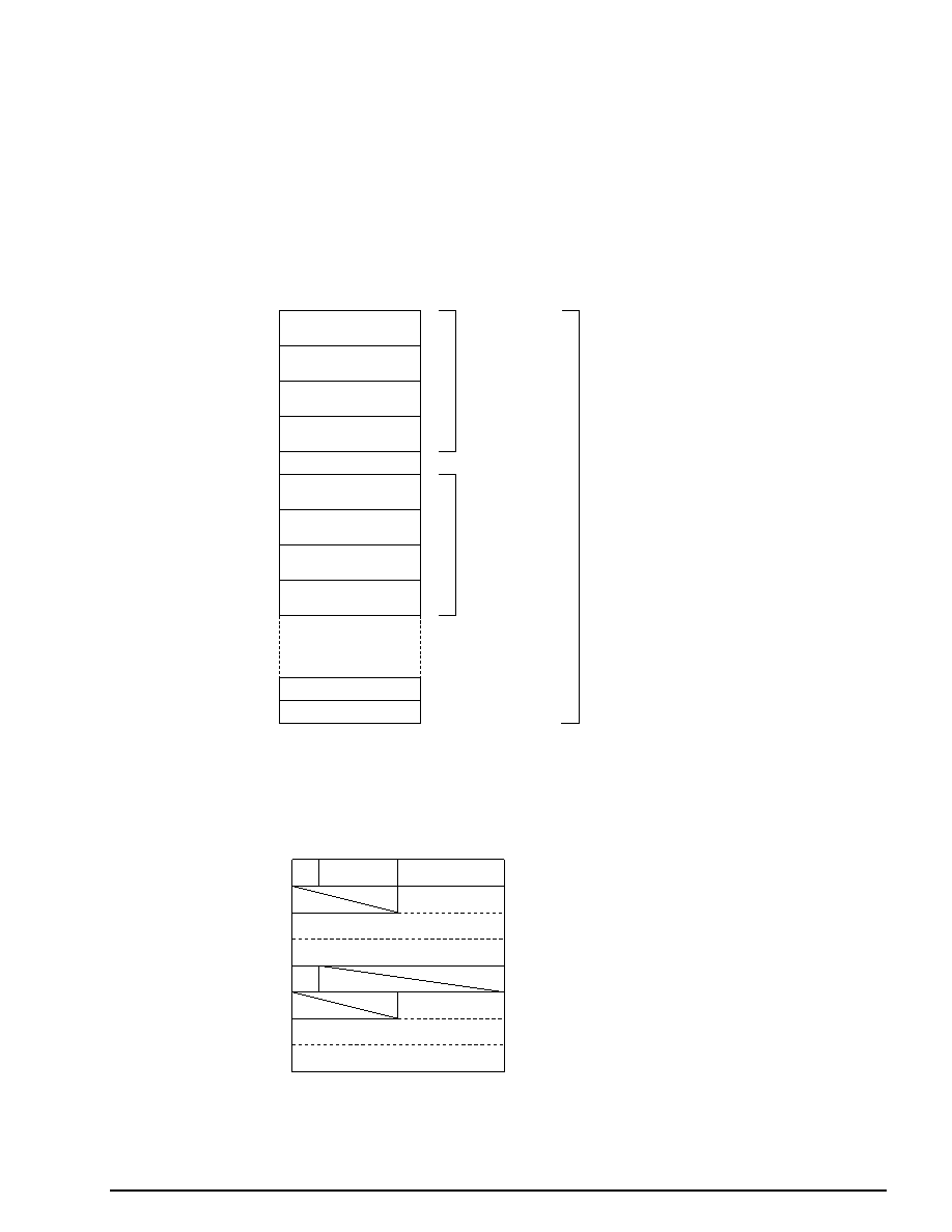
Transferring Data / Sound Data
2-3
Binary map file
The binary map file shows the load addresses in the 68000 sound CPU memory for the three
types of files described above and also the work areas used by DSP programs.
This file is loaded at address A000 in the 68000 memory.
The map can consist of up to 4096 bytes and can hold a maximum of 128 area maps. One area
map can contain up to 32 bytes of map information.
Fig 2-4 Structure of a Binary Map File
Binary map file
(4096 bytes max.)
Map 1 (8 bytes)
Map 1
Map 2
Map 2
Map 3
Map 3
Map 4
Map 4
FFh
FFh
FFh
Area map 1
(32 bytes max.)
Area map 2
end code (1 byte)
end code (1 byte)
ALL end (1 byte)
The bit image of each map (maps 1 to 4) is shown below.
Fig 2-5 Map Bit Image
0
1
2
3
4
5
6
7
7 6 5 4 3 2 1 0
E
L
Data ID
Start Address
Area Size
ID Number
0: Contains data
1: Does not contain data
0: tone bank data
1: Sequence data
2: DSP program
3: DSP work RAM
0 to 15: Data ID number
0: Data not yet transferred
1: Data has been transferred
E
Data ID
ID Number
L
|

2-4
Transferring Data / Sound Data
Fig 2-6 Example of a Binary Map File
Sound driver
In order to make sure the versions are the same, it is safest to pass the sound driver provided
with the Macintosh tools on to the programmers.
Fig 2-7 Sound Driver
Dump data file
The dump data file is a dump of memory with the files described above in items 1 to 3 loaded
into memory, from B000h to the last map data.
(However if the last data is the DSP work RAM, the dump ends with the second to last data.) In
cases where there is no need to partially load only essential banks and it is possible to load all of
the map data at one time, using the dump data file eliminates the need for loading the files
described in 1 to 3 one at a time. As a result, mistakes in the sequence in which data is loaded
are eliminated, and programming work is simplified.
The dump data file is created by the sound simulator provided with the Sega Sound Tools.
Fig 2-8 Example of a Dump Data File
|

Transferring Data / Sound Data
2-5
The diagram below shows the background music and sequence files that need to be transferred
to the programmers. Transfer either of the following groups of files to the programmers.
1. Sound driver, binary map file, dump data file (includes the tone bank data, sequence data,
and DSP program)
2. Sound driver, binary map file, tone bank data, sequence data, and DSP program
Fig 2-9 Background Music and Sequence Files Being Transferred to the Pro-
grammers
Sound driver
Binary map file
Dump data file
Tone bank data
Sequence data
DSP program
Relaying sound control numbers
The programmers use the sound control numbers to play music and sound effects in the SGL.
The sound control number is a combination of the sequence data number and the SONG number
from the sound simulator. Therefore, when transferring the files to the programmers, the sound
designer must inform the programmers of what numbers to use to produce what sounds.
Fig 2-10 Sound Control Number Being Transferred to the Programmers
Sound control number (2 bytes)
Sequence data number
SONG number
|

2-6
Transferring Data / Sound Data
PCM stream playback data
This is the PCM data used in the SGL.
Fig 2-11 Example of a PCM Data File
PCM data files are created by the sound simulator provided with the Sega Sound Tools.
The sound designer should provide the following information when passing this type of file to
the programmers.
Table 2-1 Information on PCM Data Files Being Transferred to the Programmers
File name
Sound
Stereo
Bits
Pitch
Comments
stereo.8
"10 years too early"
Stereo
8
7800
Shifts left and right
mono.16
"OK"
Monaural
16
7180
stereo.16
"Oooo"
Stereo
16
7F00
Flows from right to left
|

Transferring Data / Sound Data
2-7
Incorporating the Data
In order to incorporate the sound data files described up to this point into a program that uses
the SGL, it is necessary to convert the various individual binary data files into array data that
can be handled in C.
A sample script for performing this task in a UNIX environment is shown below.
Here we will use "sed" of "GNU".
Script name
[binary file name]
[array name]
> [output file name]
#!/bin/csh -f
echo "char $2[] = {"
od -hv $1 | cut -s -d " " -f2- | gsed 's/¥(..¥)¥(..¥) */0x¥1,0x¥2,/g'
echo "};"
Because ANSI functions can be easily used in C, create a script in C if your development
environment is PC-based.
The data is now in a form that can be incorporated into the application software. From this
point on, it can be treated in the same manner as any other data.
|

Transferring Data
3
Writing CD-ROMs
This chapter describes the method for writing user-written
games to CD-ROMs.
|

3-2
Transferring Data / Writing CD-ROMs
Flow of Work
CD-ROMs are created in the PC DOS English mode environment. As a result, file names are
subject to DOS restrictions, which means they are limited to 8 characters + 3 characters.
In order to write a user-written game to a CD-ROM, it is necessary to prepare a binary-format
IP, program, and data.
The basic flow of the CD-ROM creation process is shown in Fig 3-1. The files that are required
for CD-ROM creation are shown in Fig 3-2.
Fig 3-1 Flow of the CD-ROM Creation Process
IP creation
Build process
CD-ROM
writing process
|

Transferring Data / Writing CD-ROMs
3-3
Fig 3-2 Flow of the CD-ROM Creation Process and Files
·
·
·
IP file
Program
Data (all in binary)
Build CD-ROM image
CD-ROM writing process
·
Script file
·
TOC information file
·
CD-ROM
·
Disc image file
|

3-4
Transferring Data / Writing CD-ROMs
IP Creation
What is the "IP"?
The IP is written in the system area of the CD-ROM disc, and is used when the application uses
the Saturn boot system. The IP is required on all CD-ROM program discs. (It is not required
on data discs.)
Details on the IP are provided in "Disc Format Standards and Boot System" in the Programmer's
Guide.
IP configuration
The IP consists of the boot code and the application initial program.
The boot code consists of an ID code for the game name, a security code supplied by Sega, and
an area code.
The application initial program is positioned immediately after the area code, and is executed
immediately after the area code is executed. Thereafter, the program proceeds under the control
of the application.
Table 3-1 IP Configuration
Structure
Size
Remarks
System ID
100H
Game name, product number, version, etc.
IP
Boot Code
Security Code
D00H
Security code
Area Code
20H to 100H
Area code
Aplication Initial Program
20H to 71E0h
Initial program, file system, etc.
Details on how to create the IP are provided in "Boot System" in the Programmer's Guide.
|

Transferring Data / Writing CD-ROMs
3-5
Build
The build process is preprocessing that is performed in order to write all of the binary format
files prepared by the user (IP, program, data, etc.) onto the CD-ROM. The build process creates
the TOC information files and disc image files that are required in order to write the CD-ROM.
The build procedure is described below.
1) Prepare the files to be written to the CD-ROM
Prepare all files that are to be written to the CD-ROM on the PC hard disk. The file posi-
tions do not matter, since they will be specified in the script. The file names must be no
more than eight characters plus a period and a three-character extension, for a total of twelve
characters. The CDDA files must be arranged in Intel format. If the file is in Motorola
format, perform byte swapping. ("SWAP.EXE" is available as a byte swapping program for
DOS.)
2) Allocate the work area
Prepare a work area for creating the CD-ROM disc image. A space equal to the total file
size is required. All subsequent file creation and execution work is performed in this area.
(Change the current directory.)
3) Determine the project name
Keep the name to eight characters or less, since it will be used as the body of the MS-DOS
file names. Here, we will use "sample" as an example.
4) Create the script file
Referring to sample program 1 (Listing 3-1), use a suitable editor to create a script file. For
the file name, use the project name with the extension ".scr" added. ("sample.scr" in our
example.)
Create the script file in the directory where the VCDBUILD command (which creates the
disc configuration information file and the disc image file) will be executed.
5) Create the disc configuration information file and the disc image file
Initiate the pre-processing program "vcdbuild.exe".
Regarding the parameter, specify "vcdbuild sample" in our example.
As a result of the execution of this command, the disc configuration information file and the
disc image file are created (as "sample.rti" and "sample.dsk" in the current example.)
6) Create the TOC file
Initiate the TOC file generation program "vcdmktoc.exe". Supply the body of the RTI file
name (i.e., the project name) as the parameter: "vcdmktoc sample".
The TOC file ("sample.toc" in the example) is created as a result of the execution of this
command.
|

3-6
Transferring Data / Writing CD-ROMs
List 3-1 Sample Program 1 (Creating the Script File "sample.scr")
Disc sample.dsk
Session CDROM
LeadIn MODE1
EndLeadIn
SystemArea e:\ip.bin
Track MODE1
Volume ISO9660 sample.pvd
PrimaryVolume 0:2:16
EndPrimaryVolume
EndVolume
File ASAMPLE.BIN
FileSource e:\mode1\asample.bin
EndFileSource
EndFile
File SAMPLE1.BIN
FileSource e:\mode1\sample1.bin
EndFileSource
EndFile
File SAMPLE2.BIN
FileSource e:\mode1\sample2.bin
EndFileSource
EndFile
.....
Track CDDA
Pause 150
FileSource e:\cdda\samp_cd1.dat
EndFileSource
EndTrack
Track CDDA
Pause 150
FileSource e:\cdda\samp_cd2.dat
EndFileSource
EndTrack
Track CDDA
Pause 150
FileSource e:\cdda\samp_cd3.dat
EndFileSource
EndTrack
.....
LeadOut CDDA
Empty 500
EndLeadOut
EndSession
EndDisc
Specification of the volume descriptor
The characters appearing in bold repre
Basic volume descriptor
These four lines correspond to one fil
If there are additional files, add the
These five lines represent one CDDA tr
If there are additional tracks, add th
The CDDA specification cannot be omitt
|

Transferring Data / Writing CD-ROMs
3-7
Writing the CD-ROM
Load the CD-ROM in the CD writer and input the following CD writer command to initiate the
writing process: "segacdw.exe"
The parameters are described below:
segacdw [-s#][-i#][-t] project name
-s: Specifies the writing speed.
Specify one of the following:
1: normal speed; 2: double speed; 4: quadruple speed.
-i: Specify the SCSI ID number of the CD writer.
The default ID is "5".
-t: Write in test mode.
In test mode, the data is not written to an actual CD-ROM.
For example, the parameters could be specified in the following manner:
"segacdw -s 2 sample"
In this case, the project named "sample" is written at normal speed by the CD writer with SCSI
ID number 5.
It is best to write the data once in test mode before performing the actual writing operation and
then, if there are no errors, proceeding with the actual writing operation.
To execute test mode, specify (for example) the following:
segacdw -s 2 -t sample
|

Transferring Data
4
Data Structure
This chapter explains the model data handled by the SEGA
Saturn system, how material names are used, and the structure
of texture data.
|

4-2
Transferring Data / Data Structure
Usage of Model Data
The "model data" referred to here is a collection of three types of data: three-dimensional (x, y,
and z) coordinate point data, data on the polygons formed by four of those points, and the
polygon attribute data.
Assuming a hypothetical model name of "label", the general formats for these data types are
shown below:
Point data
POINT point_label[]={
POStoFIXED(x,y,z),
POStoFIXED(x,y,z),
POStoFIXED(x,y,z),
POStoFIXED(x,y,z),
..............
};
POINT: Point data
x, y, z: Floating-point coordinate values
The point data is indexed 0, 1, 2, and 3, in sequence from the top.
Polygon data
POLYGON polyfon_label[]={
NORMAL(x,y,z),
VERTICES(0,1,2,3),
NORMAL(x,y,z),
VERTICES(0,1,2,3),
..............
};
NORMAL: Normal vector
x, y, z: Floating-point coordinate values
VERTICES: Point data for the four vertices that form the polygon
In the case of a triangle, the last point is repeated so that the polygon still has "four" vertices.
Example: In the case where the polygon has four corners:
VERTICES(0,1,2,3)
Example: In the case where the polygon has three corners:
VERTICES(0,1,2,2)
Attribute data
ATTR attribute_label[]={
ATTRIBUTE(Plane,Sort,Texture,Color,Gouraud,Mode,Command,Option),
....... ...... ..... ...... ..... ......
};
ATTR: Attribute
Plane: Attribute determining whether front/back determination is made or not
Sort: Representative point for Z sort
Texture: Texture name (No.)
Color: Color data
Gouraud: Gouraud shading attribute
Mode: Graphics mode
Command: Polygon and texture statuses
Option: Optional functions
|

Transferring Data / Data Structure
4-3
The attributes consist of the eight parameters indicated above. The symbols actually output by
those parameters and their meanings are explained below.
[Plane]
Single_Plane:
Backside determination made
Dual_Plane:
Backside determination not made
[Sort]
SORT_MIN:
Closest point
SORT_CEN:
Mid-point
SORT_MAX:
Farthest point
[Texture]
No_Texture:
Polygon
texture name:
Texture (macro indicating the texture data)
For details, refer to "Texture Data Usage."
[Color]
No_Palet:
Texture
C_RGB(r, g, b):
Color data for a polygon
* "r," "g," and "b" stand for red, green, and blue, and represent decimal values from 0
to 31.
[Gouraud]
No_Gouraud
No gouraud shading
[Mode]
MESHon:
Mesh on
MESHoff:
Mesh off
[Command]
SprHflip:
Flip sprite horizontally
SprVflip:
Flip sprite vertically
SprHVflip:
Flip sprite horizontally and vertically
SprNoflip:
Do not flip sprite
SprPolygon:
Polygon
SprPolyLine:
Polyline
[Option]
NoOption:
No options
Of the above parameters, plane, sort, and mode are obtained through the specification of the
material name described on the next page.
|

4-4
Transferring Data / Data Structure
[MODE]
Group
Macro
Description
1
No_Windows
Accept no window restrictions (default)
Window_In
Display inside window
Window_Out
Display outside window
2
MESHoff
Normal display (default)
MESHon
Display with mesh
3
ECdis
Disable EndCode
ECenb
Enable EndCode (default)
4
SPdis
Display clear pixels (default)
SPenb
Do not display clear pixels
5
CL16Bnk
16-color color bank mode (default)
CL16Look
16-color look-up table mode
CL64Bnk
64-color color bank mode
CL128Bnk
128-color color bank mode
CL256Bnk
256-color color bank mode
CL32KRGB
32,768-color RGB mode
6
CL_Replace
Overwrite (standard) mode (default)
CL_Shadow
Shadow mode
CL_Half
Half-bright mode
CL_Trans
Semi-transparent mode
CL_Gourand
Gouraud shading mode
[Dir]
Macro
Description
sprNoflip
Display texture normally
sprHflip
Flip texture horizontally
sprVflip
Flip texture vertically
sprHVflip
Flip texture vertically and horizontally
sprPolygon
Display polygon
sprPolyLine
Display polyline
sprLine
Display straight line using first two points
[Option]
Macro
Description
UseLight
Calculate light source
UseClip
Do not display vertices outside of the screen
UsePalette
Indicates that the polygon color is palette format
Of the above parameters, "Plane", "Sort", and "Mode" are obtained by specifying them in the
material name described in the next item.
|

Transferring Data / Data Structure
4-5
Data structure
PDATA pdata_label={
point_label,n1,
point_label,n2,
attribute_label
};
Object data structure
OBJECT
object_label={
pdata_label,
TRANSLATION(x,y,z),
ROTATION(x,y,z),
SCALING(x,y,z)
object_child,
object_sibling,
};
|

4-6
Transferring Data / Data Structure
Material Name Usage
Each letter of the material name has meaning. That information is reflected directly in the
attribute data. The method is shown below.
In general the name consists of three letters, representing the following attributes in order:
[Plane][Sort][Mesh] ("[]" represents one letter; a material name is represented by three letters,
such as "SSN")
The possible attributes for each letter are:
[Plane]
S: Single_Plane
D: Dual_Plane
[Sort]
N: SORT_MIN
C: SORT_CEN
F: SORT_MAX
[Mesh]
O: MESHon
N: MESHoff
Example: If the material name is "SCN", the attribute data is as follows:
ATTRIBUTE (Single_Plane, SORT_CEN, No_Texture, C_RGB(r,g,b),
No_Gouraud, MESHoff, sprNoFlip, NoOption)
|

Transferring Data / Data Structure
4-7
Texture Data Usage
Texture data is necessary when textures are used. The texture name for the attribute "Texture"
is based on this data.
Assuming a texture DGT file named "sample.dgt":
TEXTBL(sample,hsize,vsize);
TEXDAT sample[]={
rgb,rgb,rgb,rgb,rgb,rgb,rgb,rgb,
rgb,rgb,rgb,rgb,rgb,rgb,rgb,rgb,
............................
};
TEXTBL: Texture table
sample: Indicates the label for the texture data (the file name)
hsize, vsize: Texture size ("hsize" is always a multiple of "8")
bgr: Individual pixel of texture data
Each of the three primary colors is represented by five bits, ranging in decimal value from 0 to
31.
The data format is as shown below:
1 4
4
4
3
3
3
1
1
1
2
2
2
0
0
0
B
G
R
Example:
Assume that a graphic data file named "sample.dgt" is a texture consisting of an
8
×
2 black and white checker pattern.
Fig 4-1 Checker Pattern Texture
The texture data for this texture would be as shown below:
TEXTBL(sample,8,2);
TEXDAT sample[]={
0xffff,0x8000,0xffff,0x8000,0xffff,0x8000,0xffff,0x8000,
0x8000,0xffff,0x8000,0xffff,0x8000,0xffff,0x8000,0xffff
};
The attribute data for the polygon with the material name "SCN" on which this texture is
applied is as follows:
ATTRIBUTE (Single_Plane, SORT_CEN, SAMPLE, No_Palet, No_Gouraud,
MESHoff, sprNoFlip, NoOption)
Note:
For textures, the Saturn hardware requires that the horizontal size be a multiple of
eight.
|